Bayesian 101

Our crash course into Bayesian methods. A module for "Adaptive and Bayesian Methods for Clinical Trial Design Short Course" by Dr. Alex Kaizer.

Transcript

1. Adaptive and Bayesian Methods for Clinical Trial Design Short Course Dr. Alex Kaizer A Crash Course in Bayesian (Bayes 101)
2. Paper Reference
3. Paper Motivation • Increase access and interest in the use of Bayesian methods • Introduce Bayesian concepts and contrast with frequentist approaches • Provide coding examples in R, SAS, and Stata • Use a previously completed clinical trial to illustrate how to implement and interpret the Bayesian analysis for both linear and logistic regression
4. Why Bayes? • Ability to integrate prior assumptions and knowledge • Interpretation of many summaries are more natural (e.g., posterior probabilities and credible intervals) • Usefulness in adaptive clinical trial designs • Methods to incorporate historic data through information sharing • Potential for more stable estimation properties in complex modeling problems
5. Where be the Bayes? While Bayesian statistical methods papers have increased 30% from 2010 to 2020, there was only a 1.8% increase in clinical journals. This may be due to: 1. Bayesian methods not traditionally taught in intro courses 2. Need for prior specification (can be tricky!) 3. Perception as more complex than frequentist approaches
6. Bayes Overview 𝑝𝑝 𝜽𝜽 𝒙𝒙 = 𝑝𝑝 𝒙𝒙 𝜽𝜽) 𝑝𝑝(𝒙𝒙) 𝑝𝑝 𝜽𝜽 𝒙𝒙: observed data 𝜽𝜽: parameter(s) Posterior Likelihood Prior Normalizing Constant ∫ 𝑝𝑝 𝑥𝑥 𝜃𝜃 𝑝𝑝 𝜃𝜃 𝑑𝑑𝑑𝑑
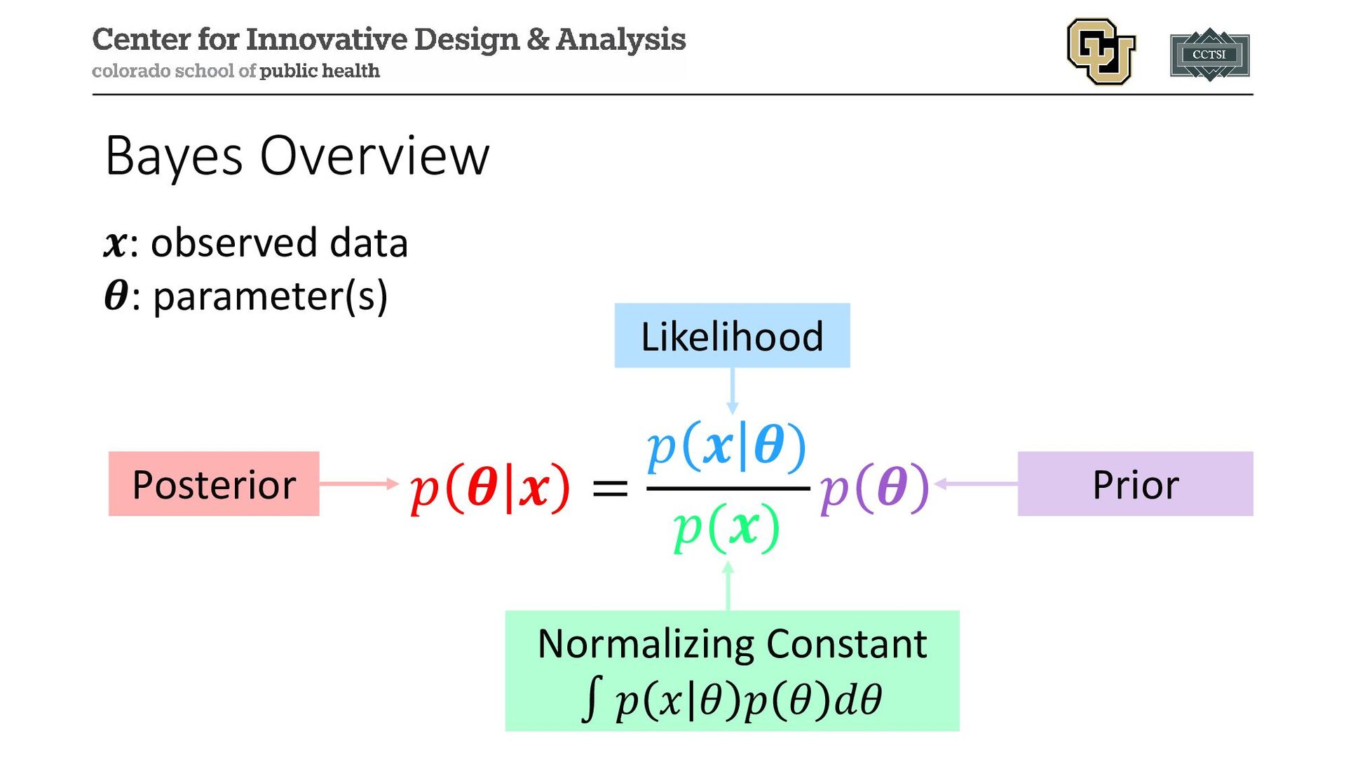
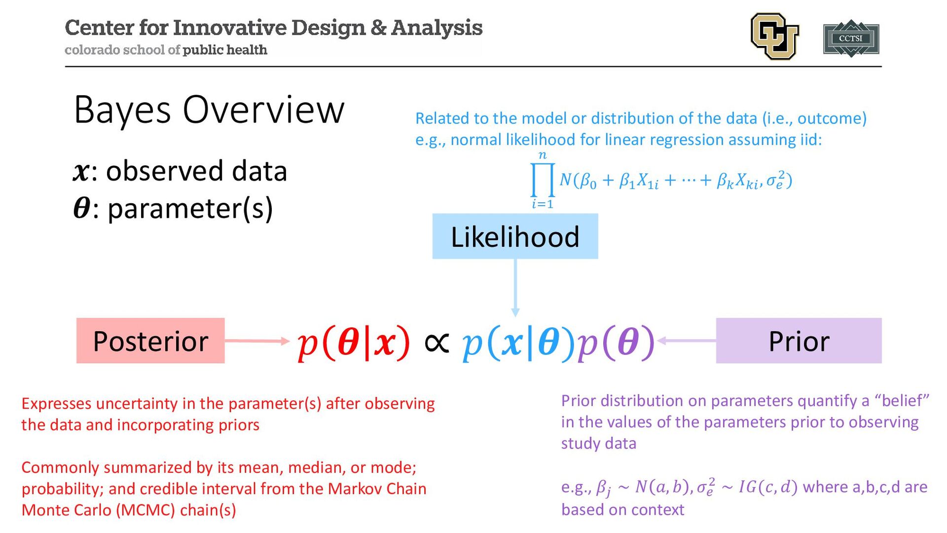
7. Bayes Overview 𝑝𝑝 𝜽𝜽 𝒙𝒙 ∝ 𝑝𝑝 𝒙𝒙 𝜽𝜽)𝑝𝑝 𝜽𝜽 𝒙𝒙: observed data 𝜽𝜽: parameter(s) Posterior Likelihood Prior Related to the model or distribution of the data (i.e., outcome) e.g., normal likelihood for linear regression assuming iid: � 𝑖𝑖=1 𝑛𝑛 𝑁𝑁(𝛽𝛽0 + 𝛽𝛽1 𝑋𝑋1𝑖𝑖 + ⋯ + 𝛽𝛽𝑘𝑘 𝑋𝑋𝑘𝑘𝑘𝑘 , 𝜎𝜎𝑒𝑒 2) Prior distribution on parameters quantify a “belief” in the values of the parameters prior to observing study data e.g., 𝛽𝛽𝑗𝑗 ∼ 𝑁𝑁 𝑎𝑎, 𝑏𝑏 , 𝜎𝜎𝑒𝑒 2 ∼ 𝐼𝐼𝐼𝐼(𝑐𝑐, 𝑑𝑑) where a,b,c,d are based on context Expresses uncertainty in the parameter(s) after observing the data and incorporating priors Commonly summarized by its mean, median, or mode; probability; and credible interval from the Markov Chain Monte Carlo (MCMC) chain(s)
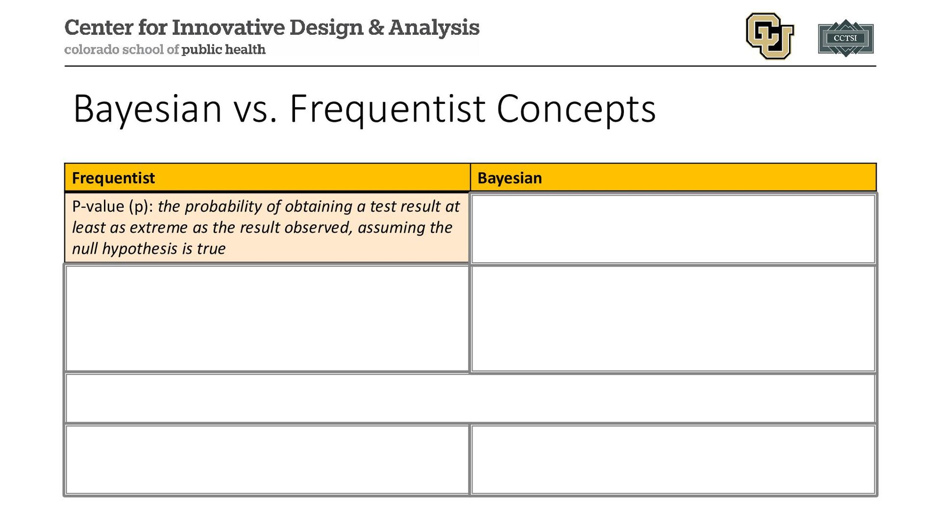
8. Bayesian vs. Frequentist Concepts Frequentist Bayesian P-value (p): the probability of obtaining a test result at least as extreme as the result observed, assuming the null hypothesis is true Posterior probability (PP): the probability of the event occurring given our observed data and prior information [it means what you think it means] 95% confidence interval (CI): we are 95% confident that the true parameter falls in this interval OR the long-run proportion of CIs that theoretically contain the true value of the parameter 95% credible interval (CrI): there is a 95% probability that the true estimate would lie within the interval [however, there are multiple ways to approach this calculation such as highest posterior density (HPD) and equal-tailed] Treats CI bounds as random variables and the parameter as a fixed value Treats CrI bounds as fixed and the estimated parameter as a random variable Conditional power: probability of rejecting the null hypothesis at the final analysis, given the current data Predictive probability [of success]: the result of averaging the conditional power over the posterior distribution of the effect size
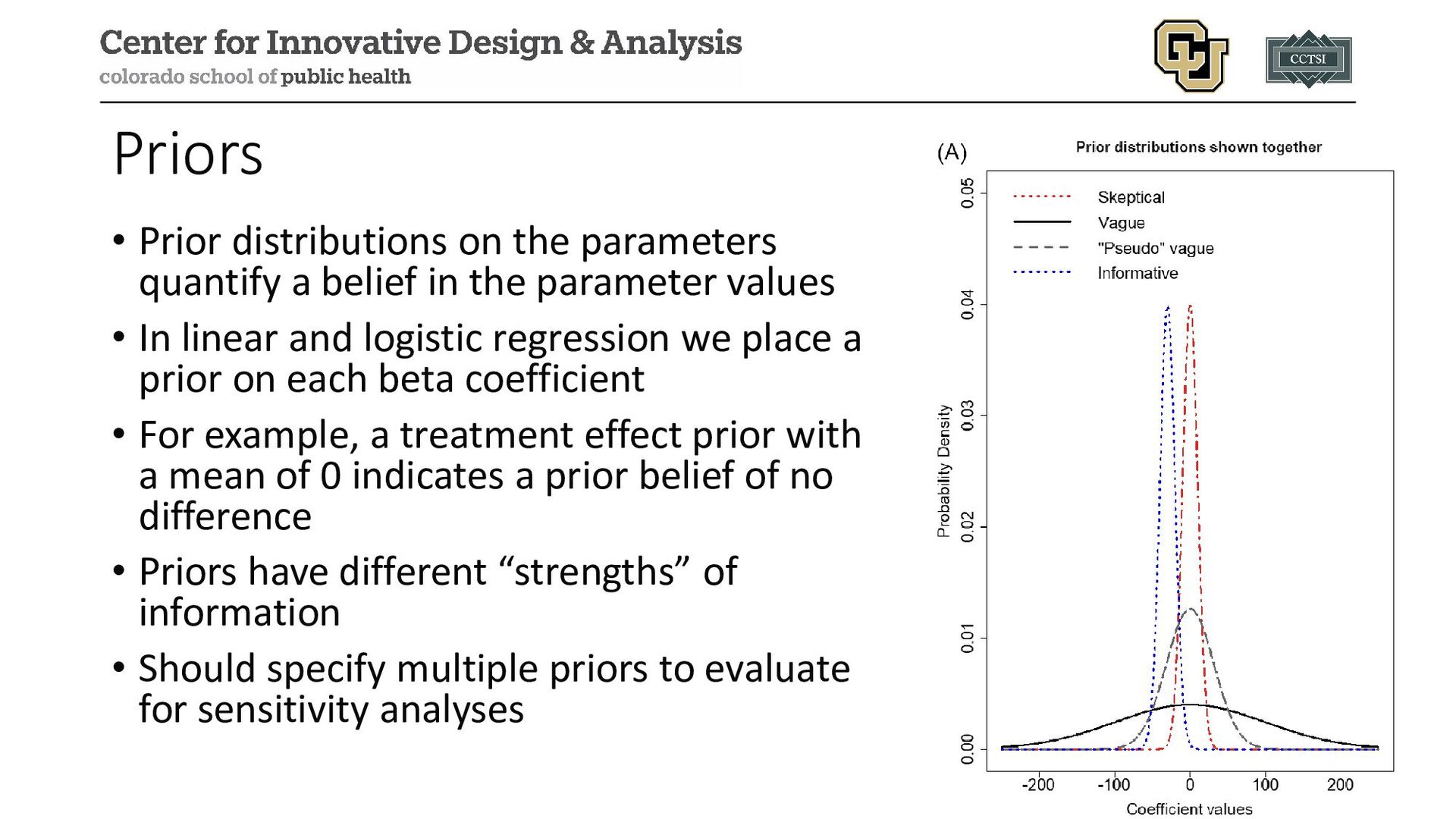
9. Priors • Prior distributions on the parameters quantify a belief in the parameter values • In linear and logistic regression we place a prior on each beta coefficient • For example, a treatment effect prior with a mean of 0 indicates a prior belief of no difference • Priors have different “strengths” of information • Should specify multiple priors to evaluate for sensitivity analyses
10. Posterior Estimation • The posterior is used to estimate our parameter(s) of interest and conduct any statistical inference • In many cases the posterior is not a known distribution that can be mathematically derived, instead we must use algorithms (e.g., Markov Chain Monte Carlo methods) to sample from this distribution
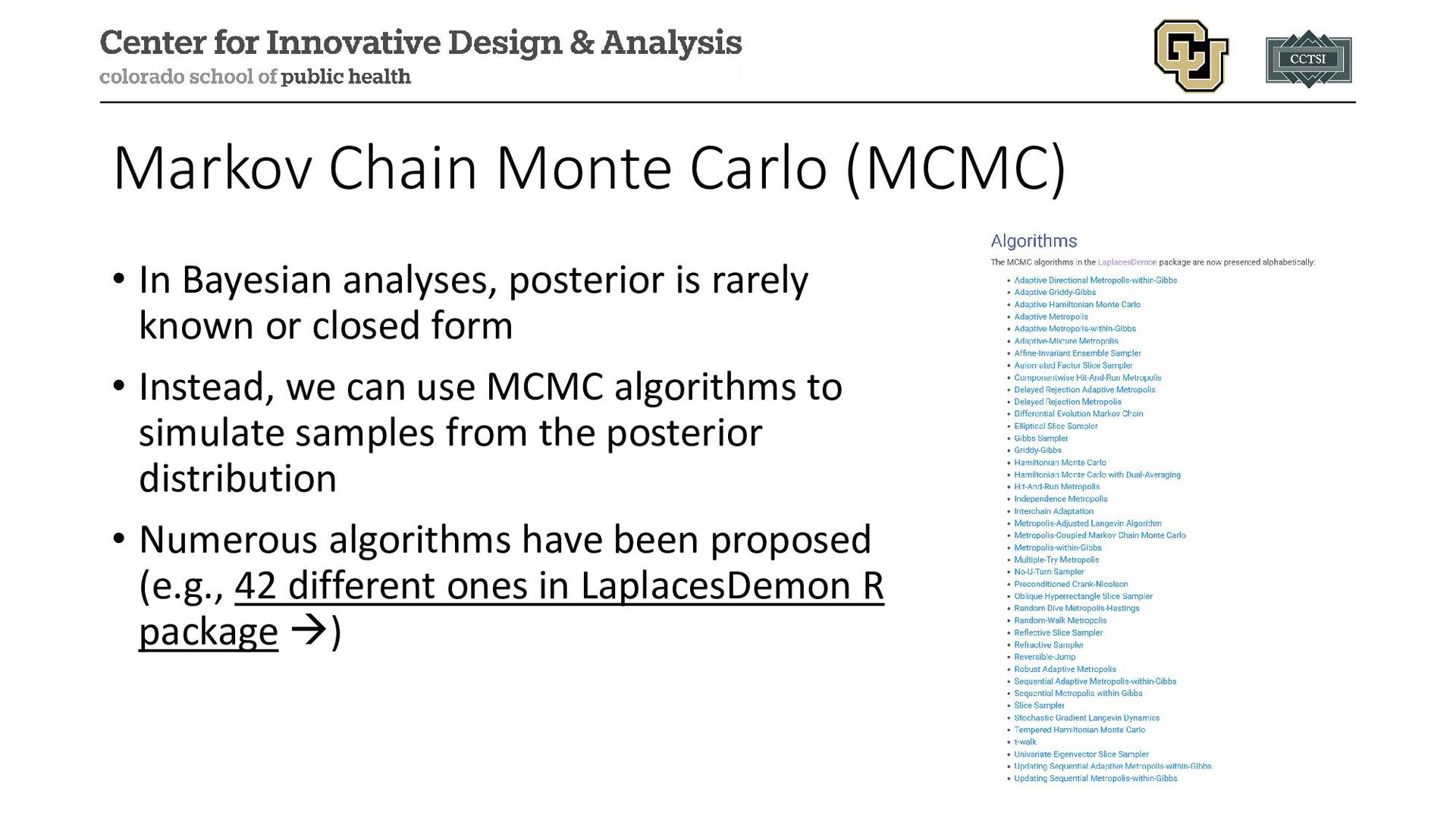
11. Markov Chain Monte Carlo (MCMC) • In Bayesian analyses, posterior is rarely known or closed form • Instead, we can use MCMC algorithms to simulate samples from the posterior distribution • Numerous algorithms have been proposed (e.g., 42 different ones in LaplacesDemon R package )
12. MCMC cont. • Many software packages (e.g., PROC MCMC in SAS, brms in R) include default MCMC algorithms to avoid users having to code their own • Output from MCMC algorithms are usually rectangular datasets with a column for each chain and a row for each iteration • Chains are separate instances of the MCMC algorithm, often with different initial values • Burn-in periods are the first “X” of each chain discarded to provide time for convergence
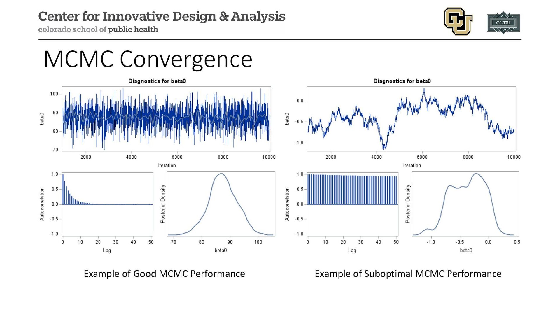
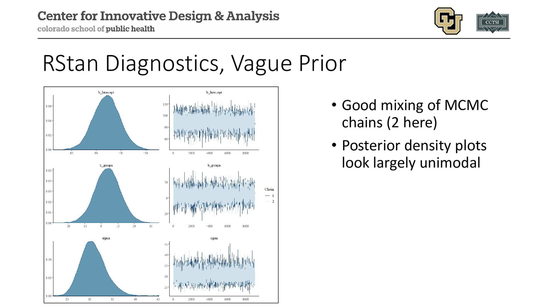
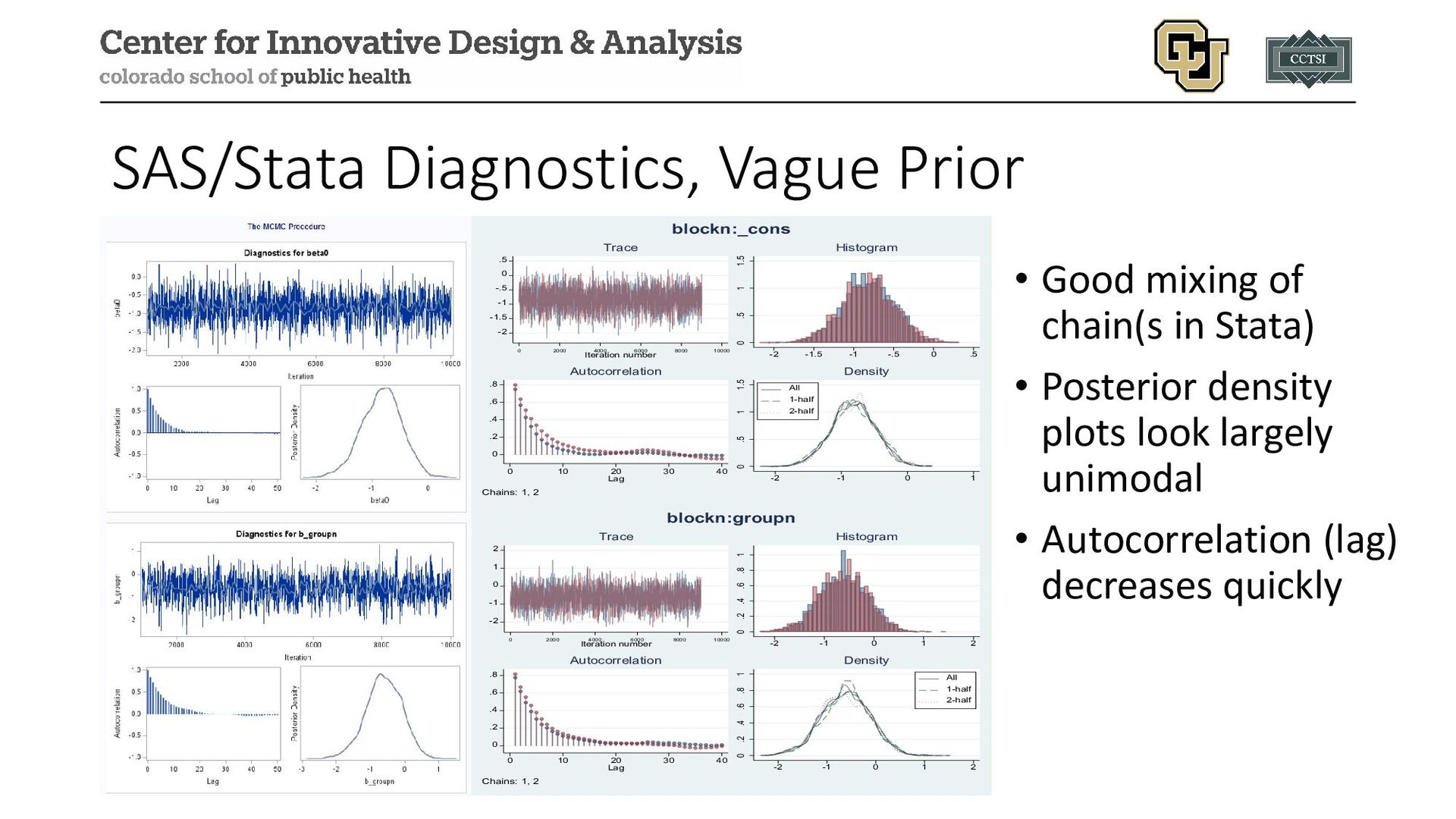
13. MCMC Diagnostics • While not the focus of this talk, we note a few diagnostic tools: • Trace plots • Autocorrelation plots • Density plots • Numerical diagnostics • Major goal is to assess whether simulation converged to the posterior distribution or if changes need to be made
14. MCMC Convergence Example of Good MCMC Performance Example of Suboptimal MCMC Performance
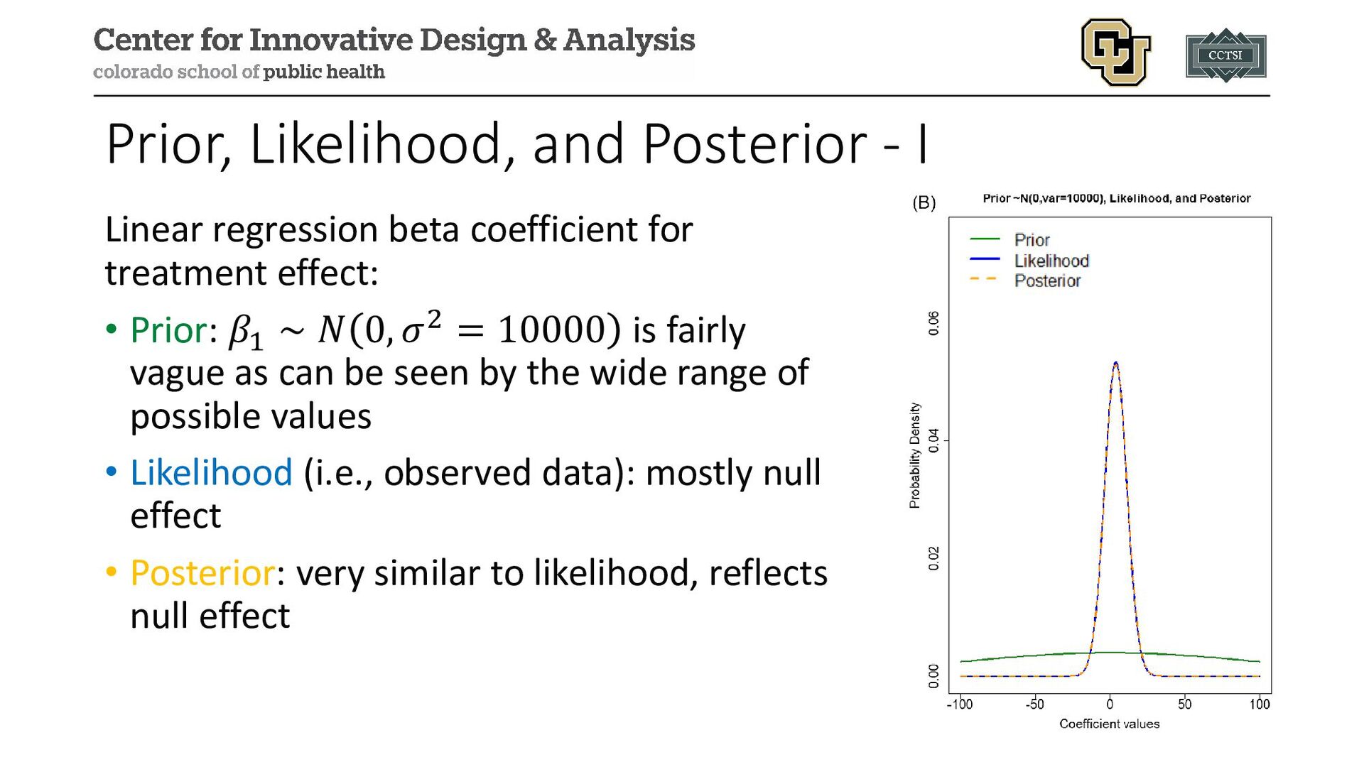
15. Prior, Likelihood, and Posterior - I Linear regression beta coefficient for treatment effect: • Prior: 𝛽𝛽1 ∼ 𝑁𝑁 0, 𝜎𝜎2 = 10000 is fairly vague as can be seen by the wide range of possible values • Likelihood (i.e., observed data): mostly null effect • Posterior: very similar to likelihood, reflects null effect
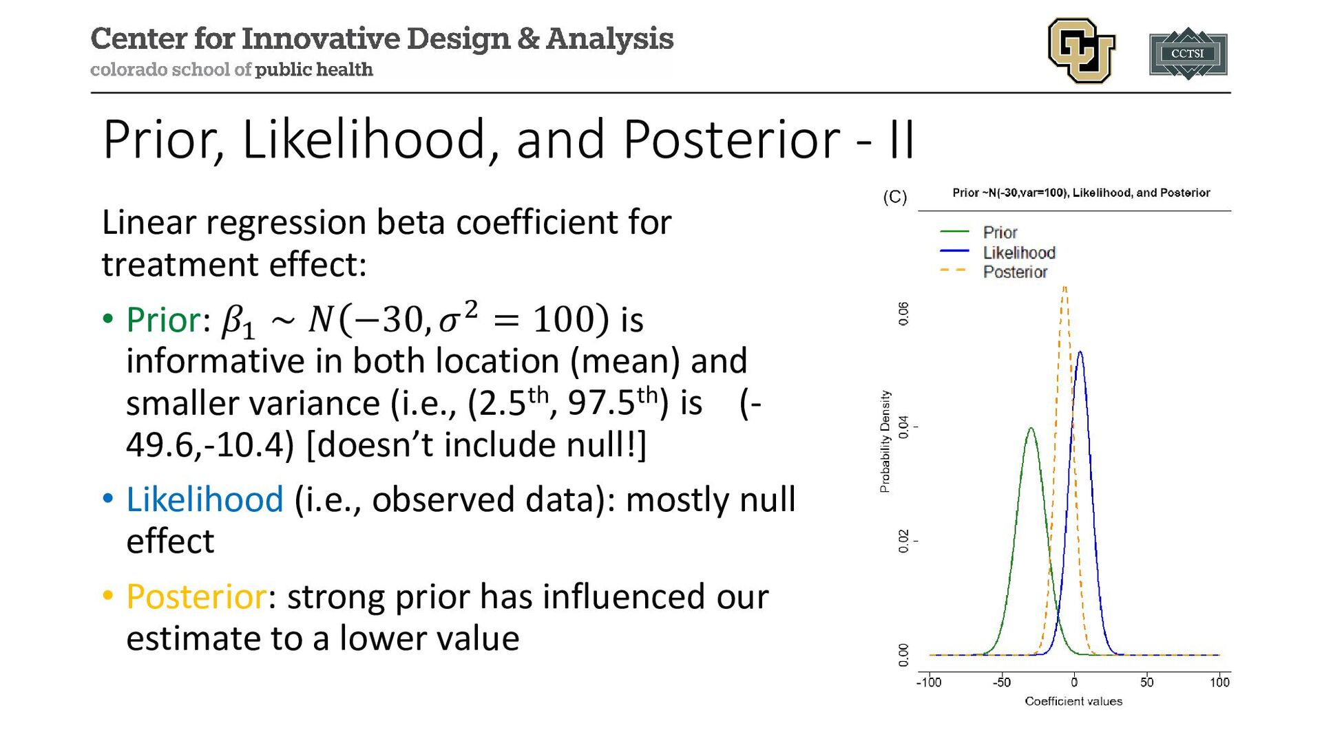
16. Prior, Likelihood, and Posterior - II Linear regression beta coefficient for treatment effect: • Prior: 𝛽𝛽1 ∼ 𝑁𝑁 −30, 𝜎𝜎2 = 100 is informative in both location (mean) and smaller variance (i.e., (2.5th, 97.5th) is (- 49.6,-10.4) [doesn’t include null!] • Likelihood (i.e., observed data): mostly null effect • Posterior: strong prior has influenced our estimate to a lower value
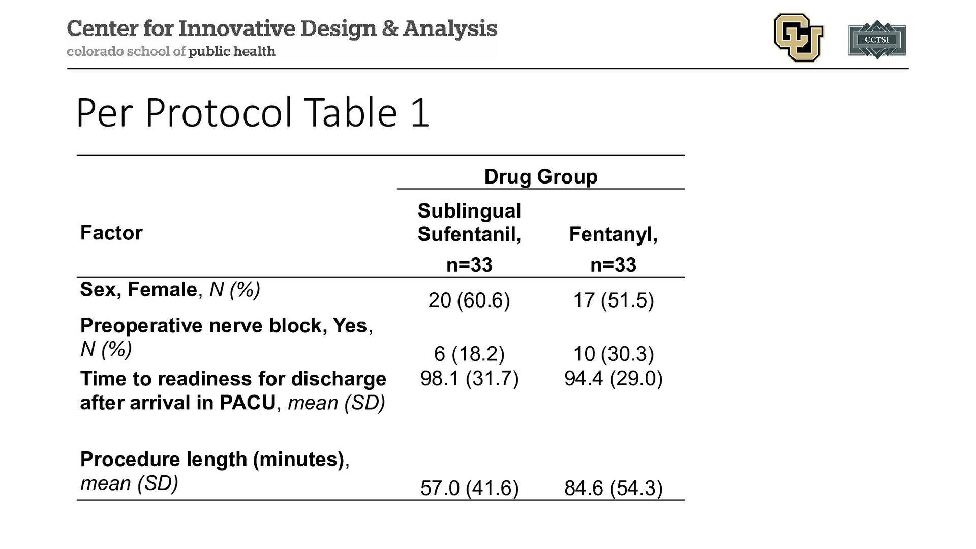
17. JCTS Data Illustration • Small clinical trial from anesthesiologist collaborators • Comparing sublingual sufentanil to standard of care IV fentanyl • 75 total randomized, but we use the 66 per protocol population to illustrate the analysis (and to avoid duplicating past work) • Continuous outcome of time to readiness for discharge after arrival in the post-anesthesia care unit (minutes) • Categorical outcome of preoperative nerve block used
18. Per Protocol Table 1 Drug Group Factor Sublingual Sufentanil, n=33 Fentanyl, n=33 Sex, Female, N (%) 20 (60.6) 17 (51.5) Preoperative nerve block, Yes, N (%) 6 (18.2) 10 (30.3) Time to readiness for discharge after arrival in PACU, mean (SD) 98.1 (31.7) 94.4 (29.0) Procedure length (minutes), mean (SD) 57.0 (41.6) 84.6 (54.3)
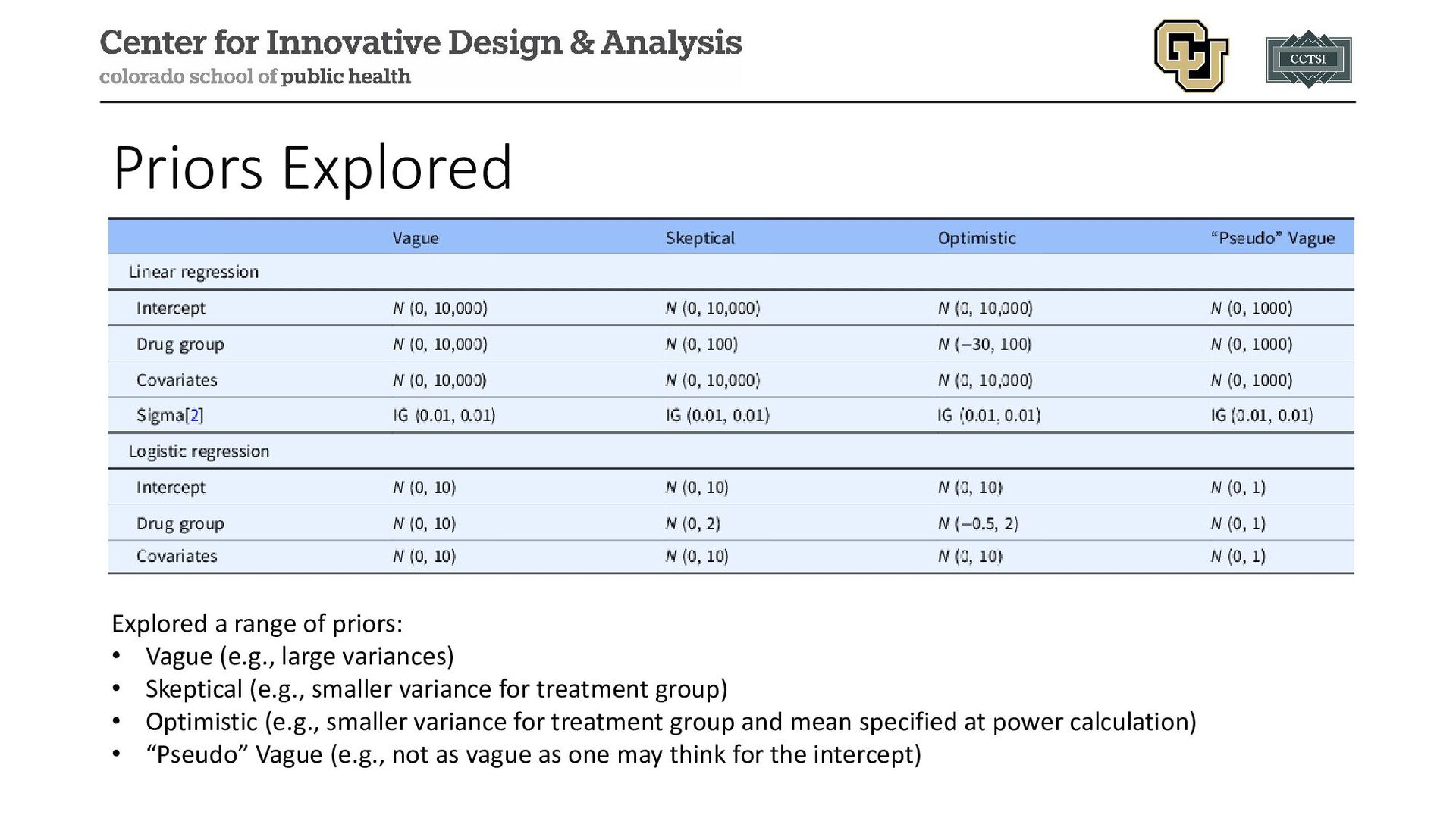
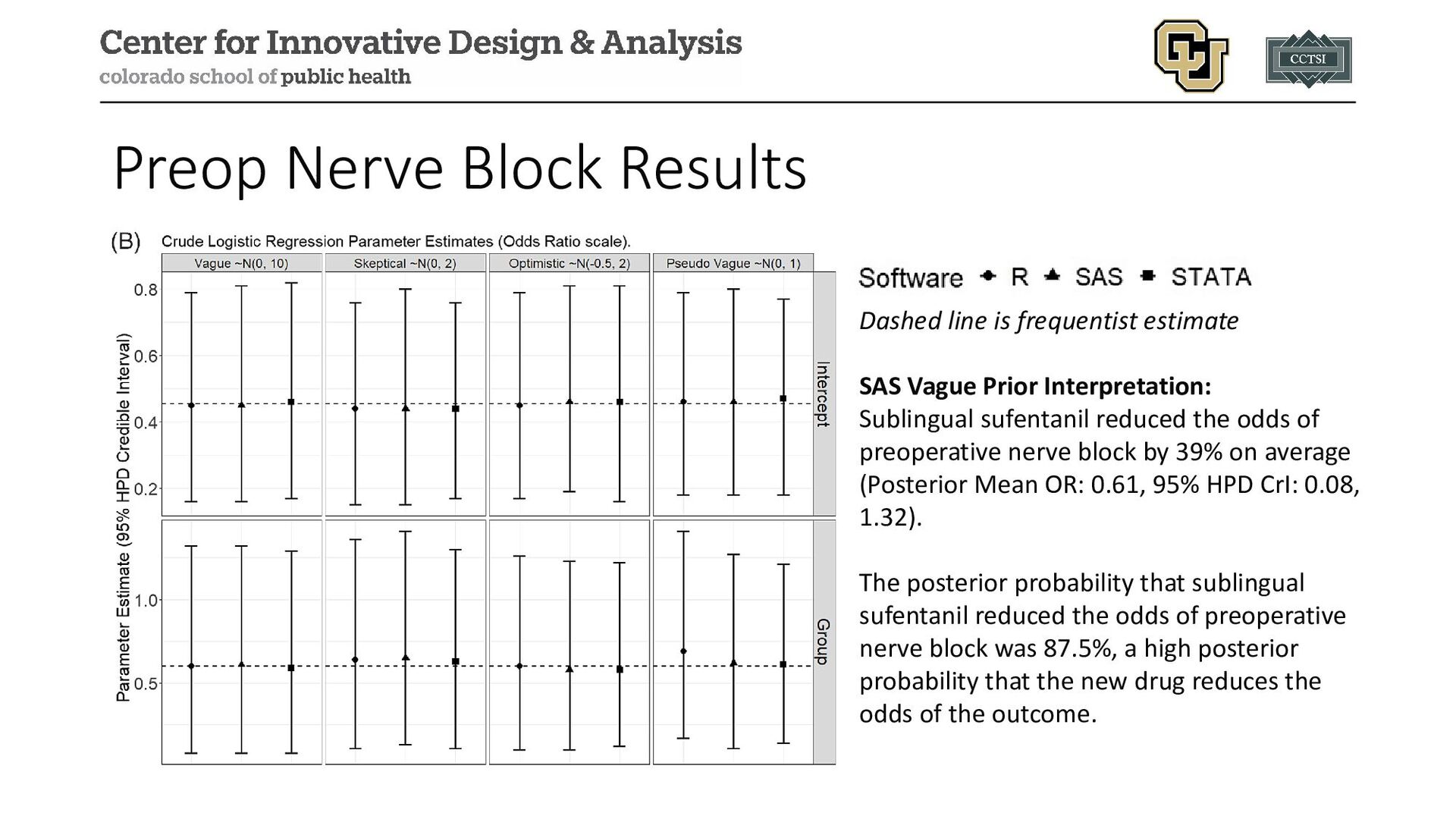
19. Priors Explored Explored a range of priors: • Vague (e.g., large variances) • Skeptical (e.g., smaller variance for treatment group) • Optimistic (e.g., smaller variance for treatment group and mean specified at power calculation) • “Pseudo” Vague (e.g., not as vague as one may think for the intercept)
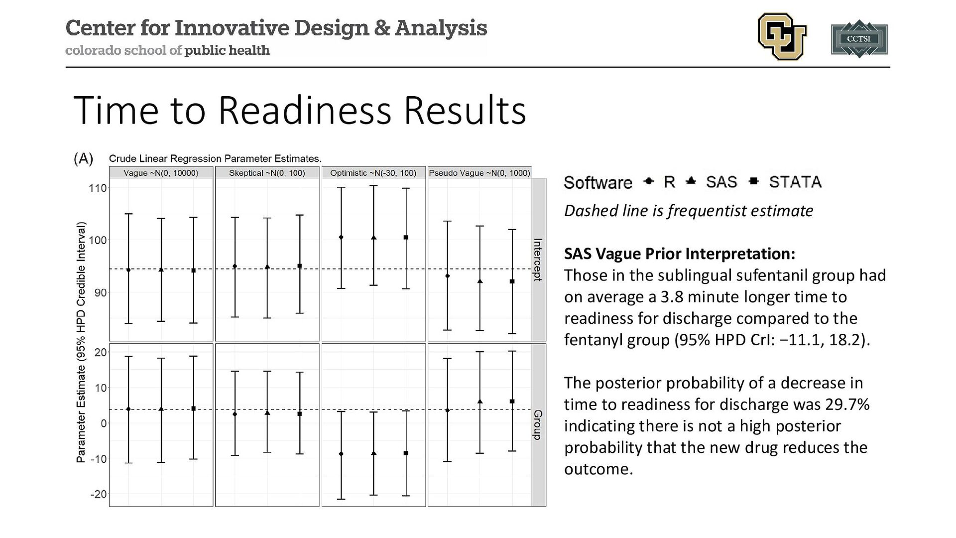
20. Time to Readiness Results Dashed line is frequentist estimate SAS Vague Prior Interpretation: Those in the sublingual sufentanil group had on average a 3.8 minute longer time to readiness for discharge compared to the fentanyl group (95% HPD CrI: −11.1, 18.2). The posterior probability of a decrease in time to readiness for discharge was 29.7% indicating there is not a high posterior probability that the new drug reduces the outcome.
21. RStan Diagnostics, Vague Prior • Good mixing of MCMC chains (2 here) • Posterior density plots look largely unimodal
22. Preop Nerve Block Results Dashed line is frequentist estimate SAS Vague Prior Interpretation: Sublingual sufentanil reduced the odds of preoperative nerve block by 39% on average (Posterior Mean OR: 0.61, 95% HPD CrI: 0.08, 1.32). The posterior probability that sublingual sufentanil reduced the odds of preoperative nerve block was 87.5%, a high posterior probability that the new drug reduces the odds of the outcome.
23. SAS/Stata Diagnostics, Vague Prior • Good mixing of chain(s in Stata) • Posterior density plots look largely unimodal • Autocorrelation (lag) decreases quickly -2 -1.5 -1 -.5 0 .5 0 2000 4000 6000 8000 10000 Iteration number Trace 0 .5 1 1.5 -2 -1.5 -1 -.5 0 .5 Histogram 0 .2 .4 .6 .8 0 10 20 30 40 Lag Autocorrelation 0 .5 1 1.5 -2 -1 0 1 All 1-half 2-half Density Chains: 1, 2 blockn:_cons -2 -1 0 1 2 0 2000 4000 6000 8000 10000 Iteration number Trace 0 .2 .4 .6 .8 1 -2 -1 0 1 2 Histogram 0 .2 .4 .6 .8 0 10 20 30 40 Lag Autocorrelation 0 .2 .4 .6 .8 1 -2 -1 0 1 2 All 1-half 2-half Density Chains: 1, 2 blockn:groupn
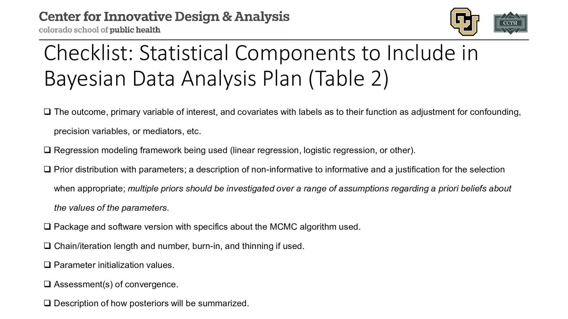
24. Checklist: Statistical Components to Include in Bayesian Data Analysis Plan (Table 2)  The outcome, primary variable of interest, and covariates with labels as to their function as adjustment for confounding, precision variables, or mediators, etc.  Regression modeling framework being used (linear regression, logistic regression, or other).  Prior distribution with parameters; a description of non-informative to informative and a justification for the selection when appropriate; multiple priors should be investigated over a range of assumptions regarding a priori beliefs about the values of the parameters.  Package and software version with specifics about the MCMC algorithm used.  Chain/iteration length and number, burn-in, and thinning if used.  Parameter initialization values.  Assessment(s) of convergence.  Description of how posteriors will be summarized.
25. Case Study 25
26. Example of More Complex Analysis
27. Motivation: COVID-19 • Declared a global pandemic by the World Health Organization in March 2020 • Need to identify potential interventions (both novel and existing drugs for other conditions) • Many unknowns in 2020 when study was designed (planning April 2020, first patient enrolled June 2020) • Continual evolution of new variants 27
28. Clinical Trial: Bayesian Example Name: TRial of Early Antiviral Therapies during Non-hospitalized Outpatient Window (TREAT NOW; NCT04372628) Design: multi-center, double-blind, randomized, placebo-controlled, decentralized trial; initial design as a platform trial Population: outpatient treatment of adults with COVID-19 within 7 days of positive test Purpose: compare existing anti-viral therapies to a placebo arm to identify if any are effective in treating COVID-19; initial anti-viral therapies included lopinavir/ritonavir and hydroxychloroquine 28
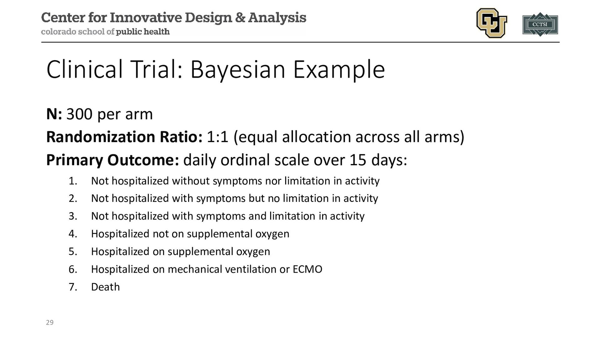
29. Clinical Trial: Bayesian Example N: 300 per arm Randomization Ratio: 1:1 (equal allocation across all arms) Primary Outcome: daily ordinal scale over 15 days: 1. Not hospitalized without symptoms nor limitation in activity 2. Not hospitalized with symptoms but no limitation in activity 3. Not hospitalized with symptoms and limitation in activity 4. Hospitalized not on supplemental oxygen 5. Hospitalized on supplemental oxygen 6. Hospitalized on mechanical ventilation or ECMO 7. Death 29
30. Primary Outcome
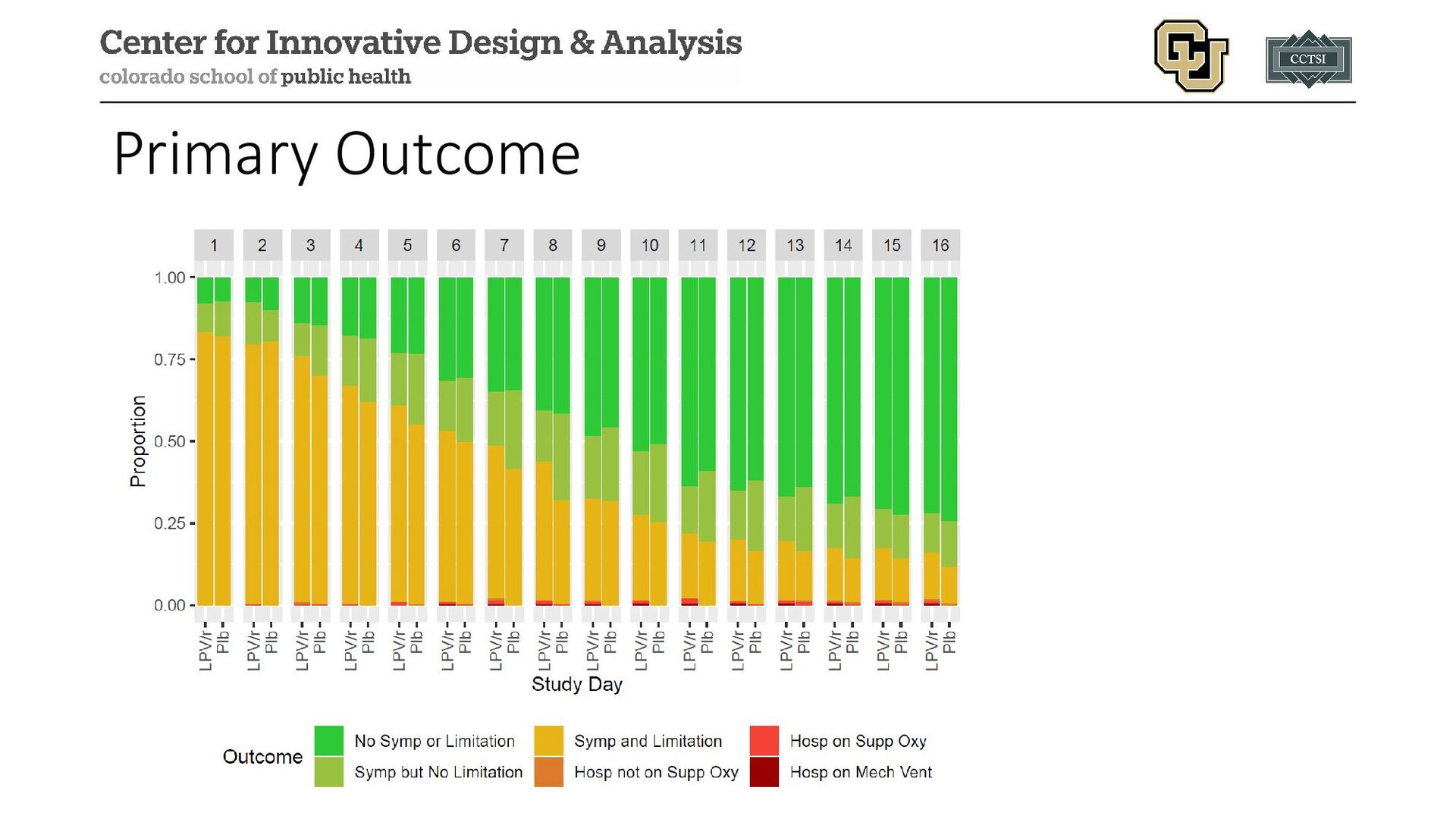
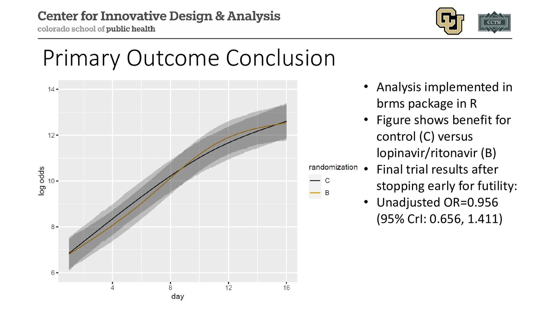
31. Primary Outcome Conclusion • Analysis implemented in brms package in R • Figure shows benefit for control (C) versus lopinavir/ritonavir (B) • Final trial results after stopping early for futility: • Unadjusted OR=0.956 (95% CrI: 0.656, 1.411)
32. Module Conclusions • JCTS paper meant to be hands-on guide with code examples of how to implement Bayesian approaches to translational research projects • TREAT NOW showed example of a more complex trial with Bayesian methods and primary form of analysis • In many cases, Bayesian and frequentist methods are not that different but important philosophical differences exist
33. References • Gunn-Sandell, Lauren B., et al. "A practical guide to adopting Bayesian analyses in clinical research." Journal of Clinical and Translational Science 8.1 (2024): e3. • Kaizer, Alexander M., et al. "Trial of Early Antiviral Therapies during Non-hospitalized Outpatient Window (TREAT NOW) for COVID-19: a summary of the protocol and analysis plan for a decentralized randomized controlled trial." Trials 23.1 (2022): 273. • Kaizer, Alexander M., et al. "Lopinavir/ritonavir for treatment of non-hospitalized patients with COVID-19: a randomized clinical trial." International Journal of Infectious Diseases 128 (2023): 223-229.
34. Contact Info: • Email: • alex.kaizer@cuanschutz.edu • Website: www.alexkaizer.com • GitHub: alexbiostats