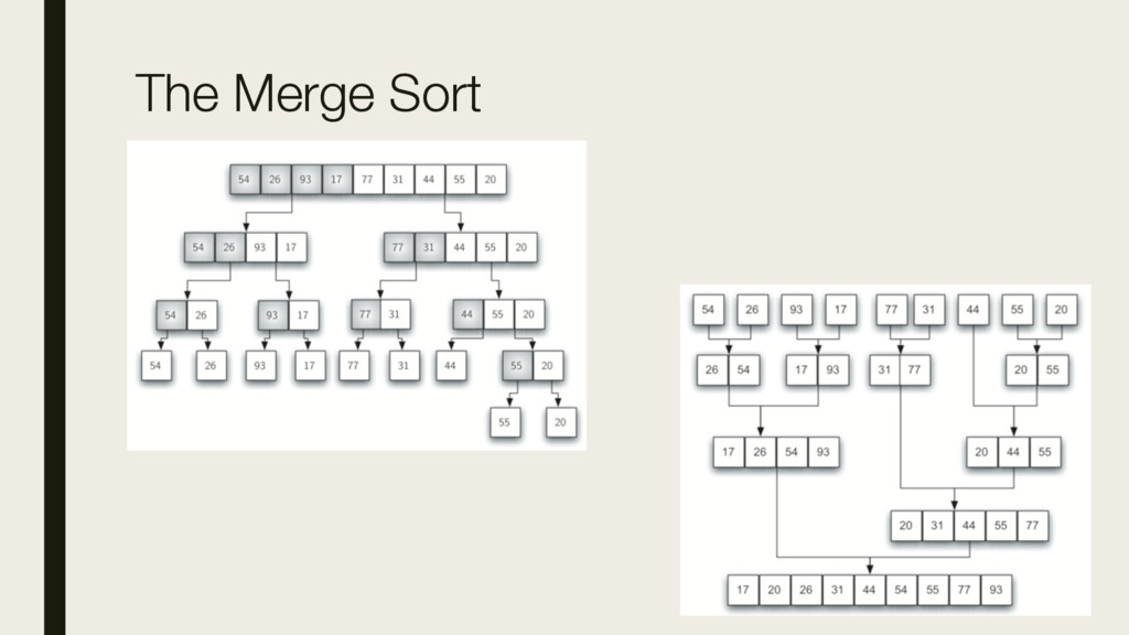
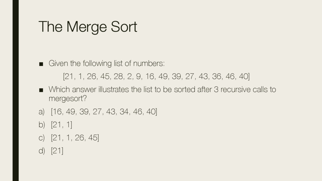
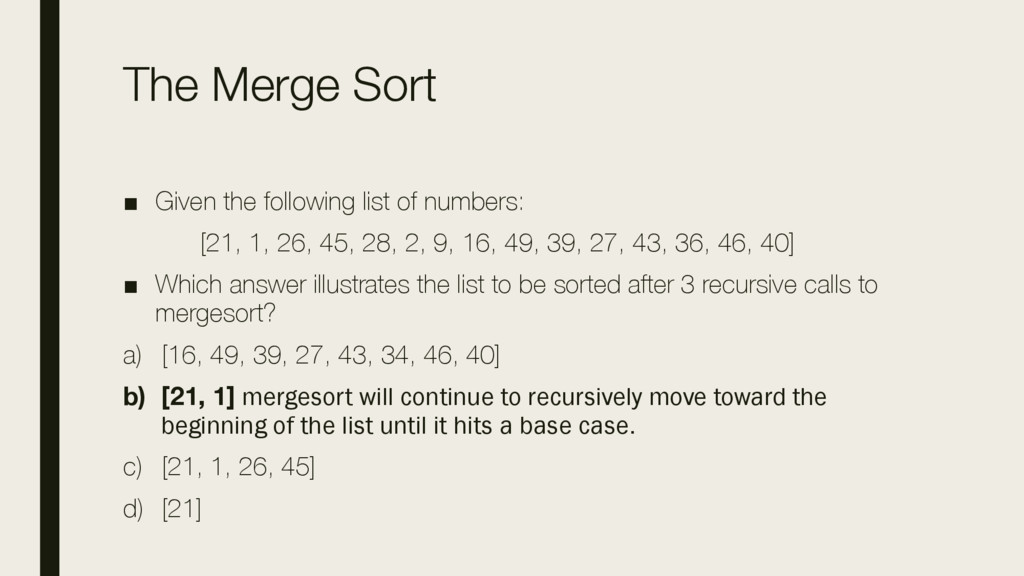
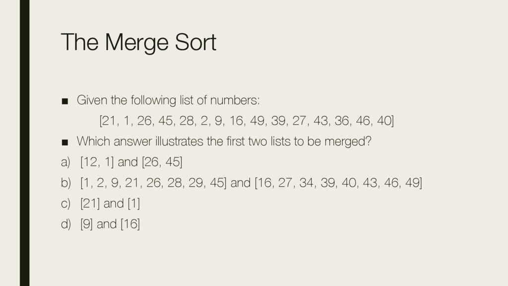
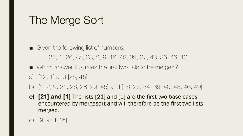
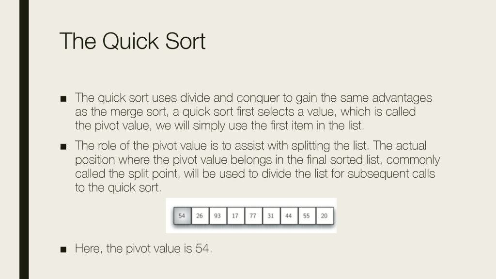
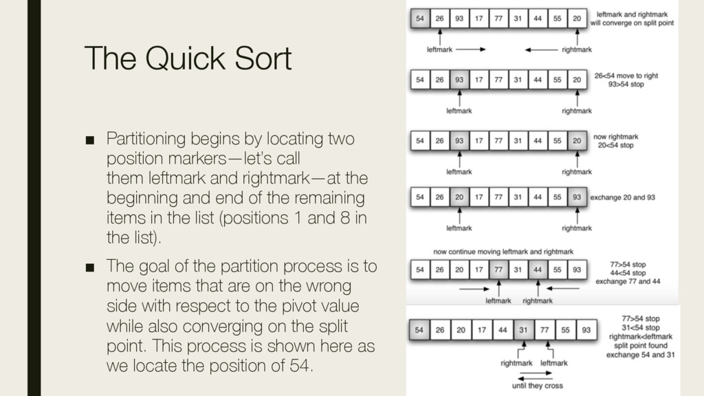
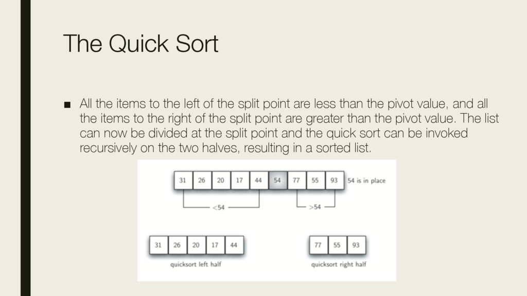
[21, 1, 26, 45, 28, 2, 9, 16, 49, 39, 27, 43, 36, 46, 40] ▪ Which answer illustrates the first two lists to be merged? a) [12, 1] and [26, 45] b) [1, 2, 9, 21, 26, 28, 29, 45] and [16, 27, 34, 39, 40, 43, 46, 49] c) [21] and [1] The lists [21] and [1] are the first two base cases encountered by mergesort and will therefore be the first two lists merged. d) [9] and [16]