Control-flow Discovery from Event Streams

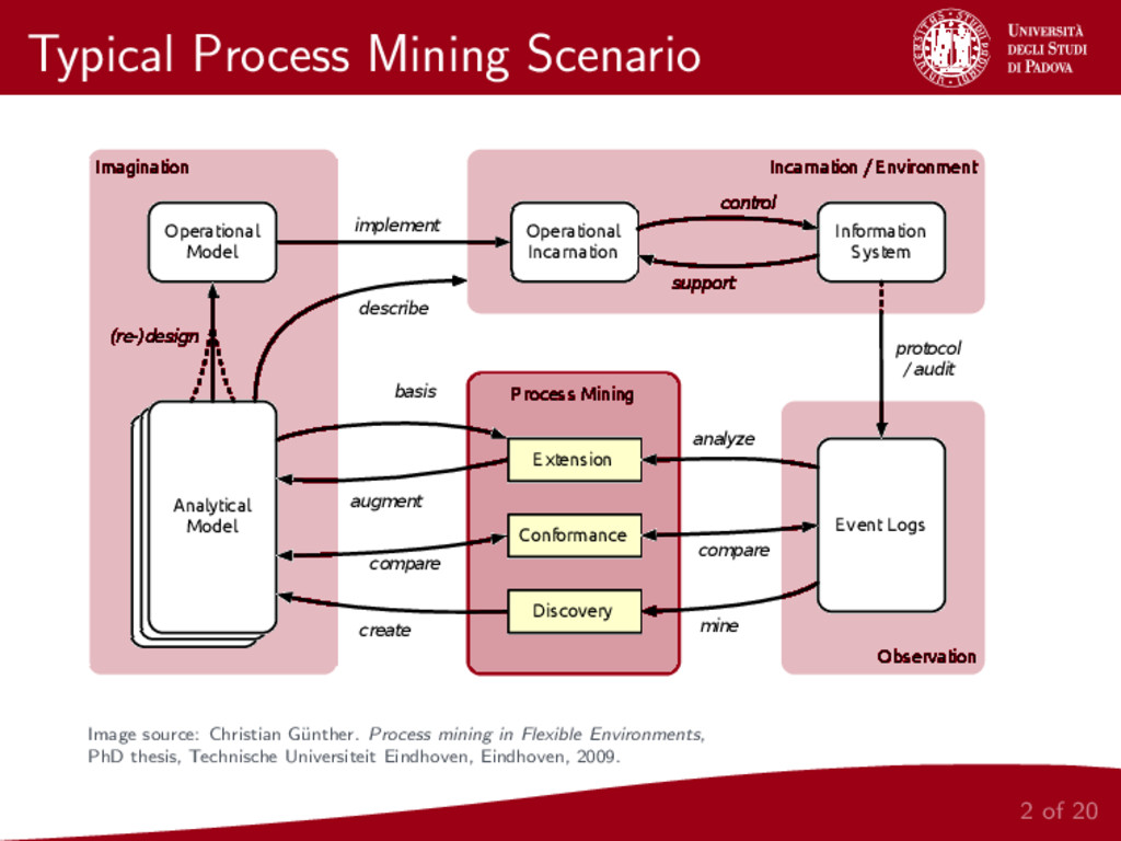
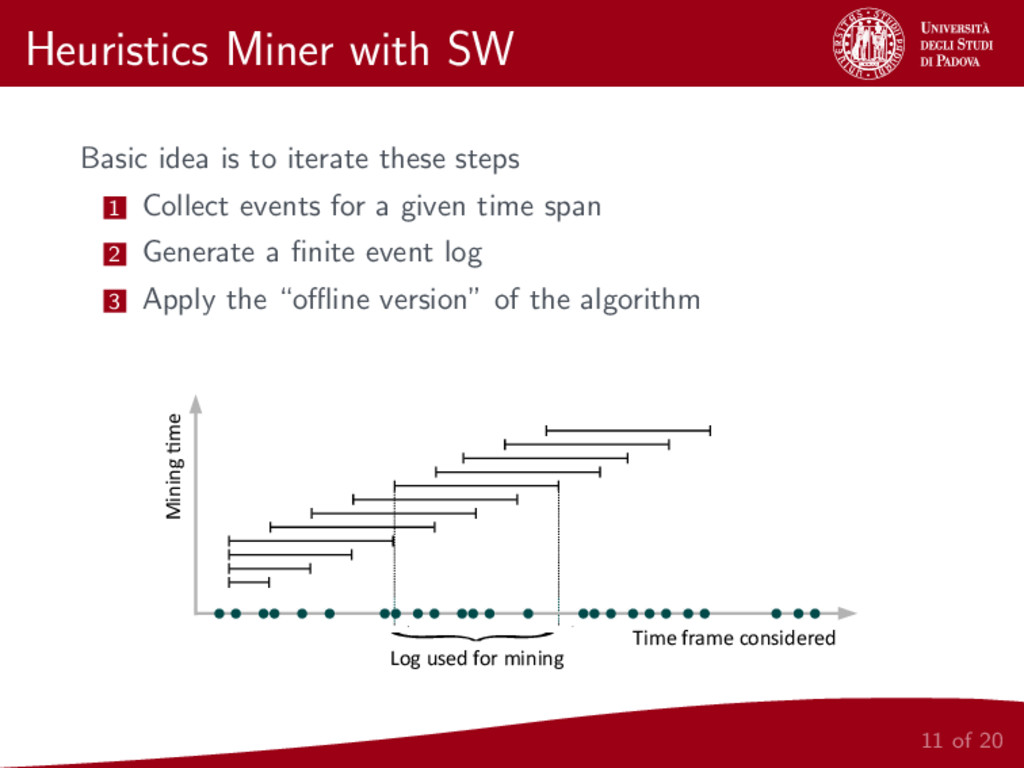
Process Mining represents an important research field that connects Business Process Modeling and Data Mining. One of the most prominent task of Process Mining is the discovery of a control-flow starting from event logs. This paper focuses on the important problem of control-flow discovery starting from a stream of event data. We propose to adapt Heuristics Miner, one of the most effective control-flow discovery algorithms, to the treatment of streams of event data.

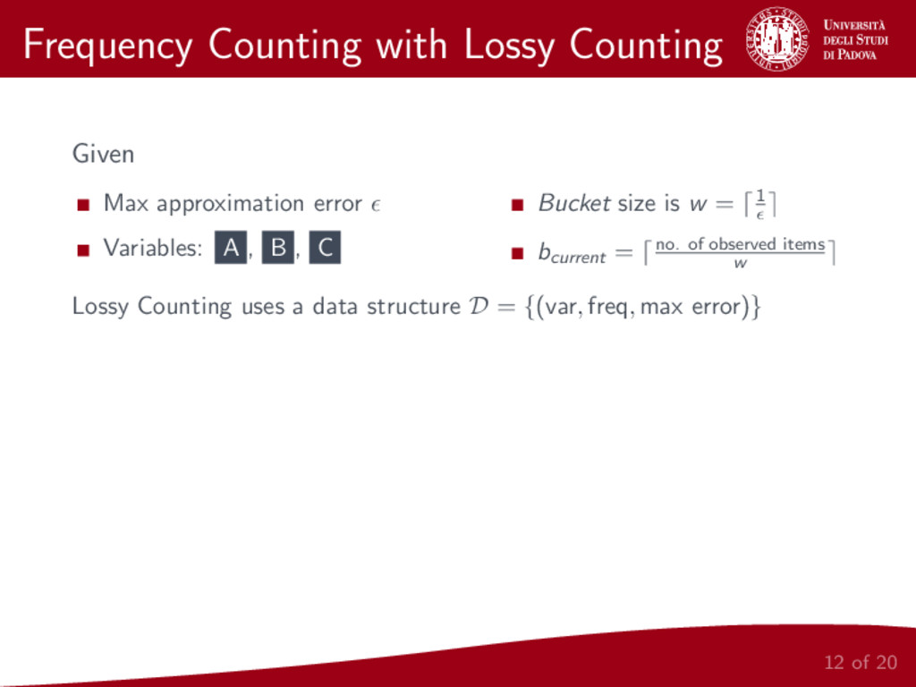
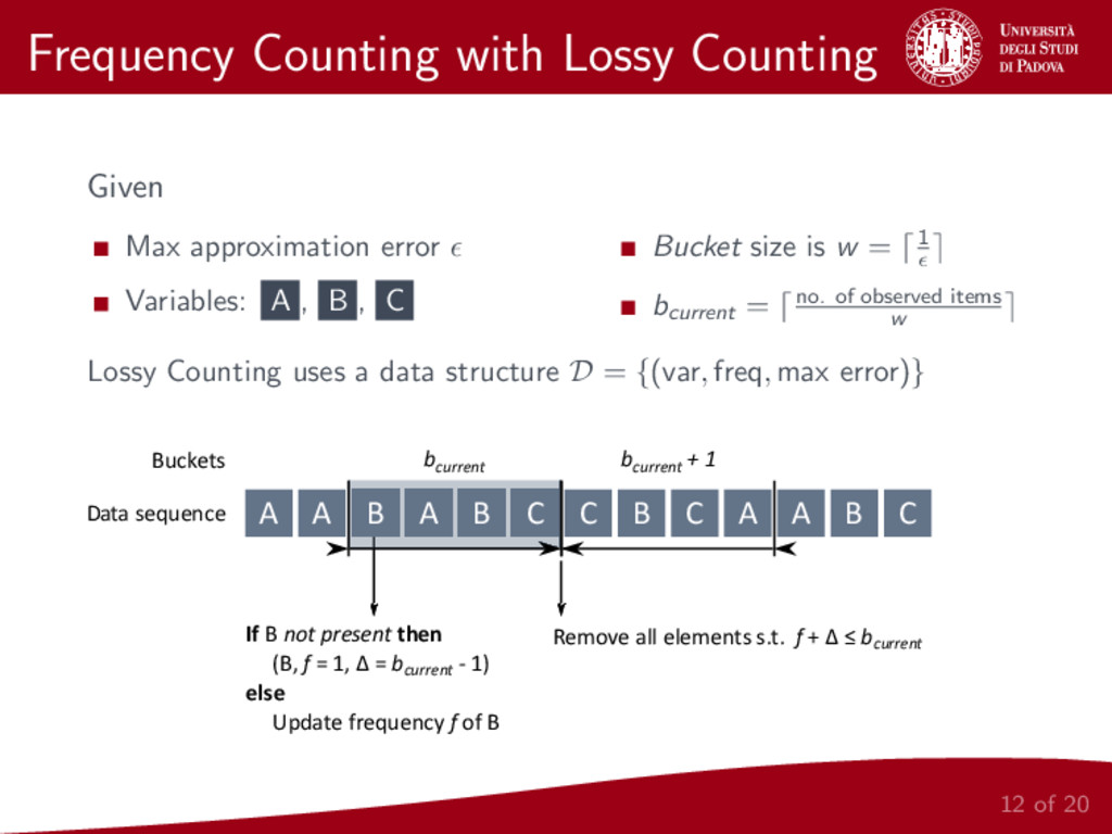
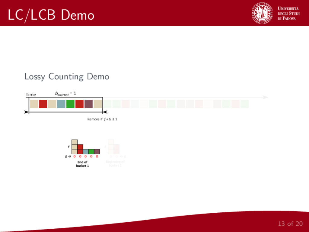
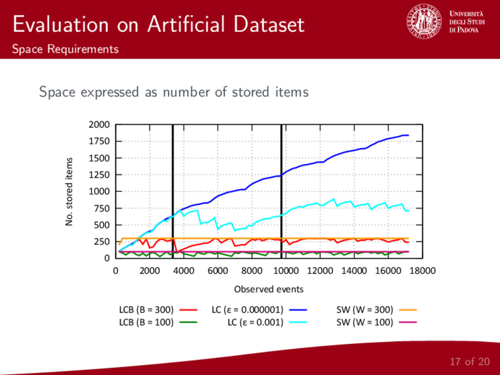
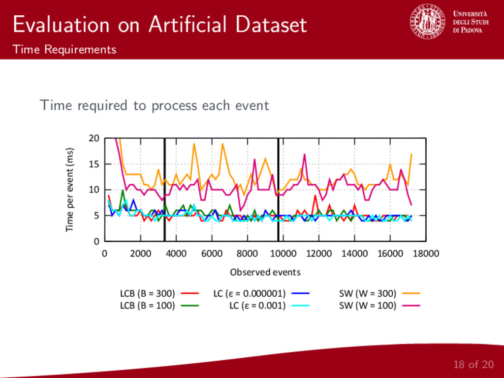
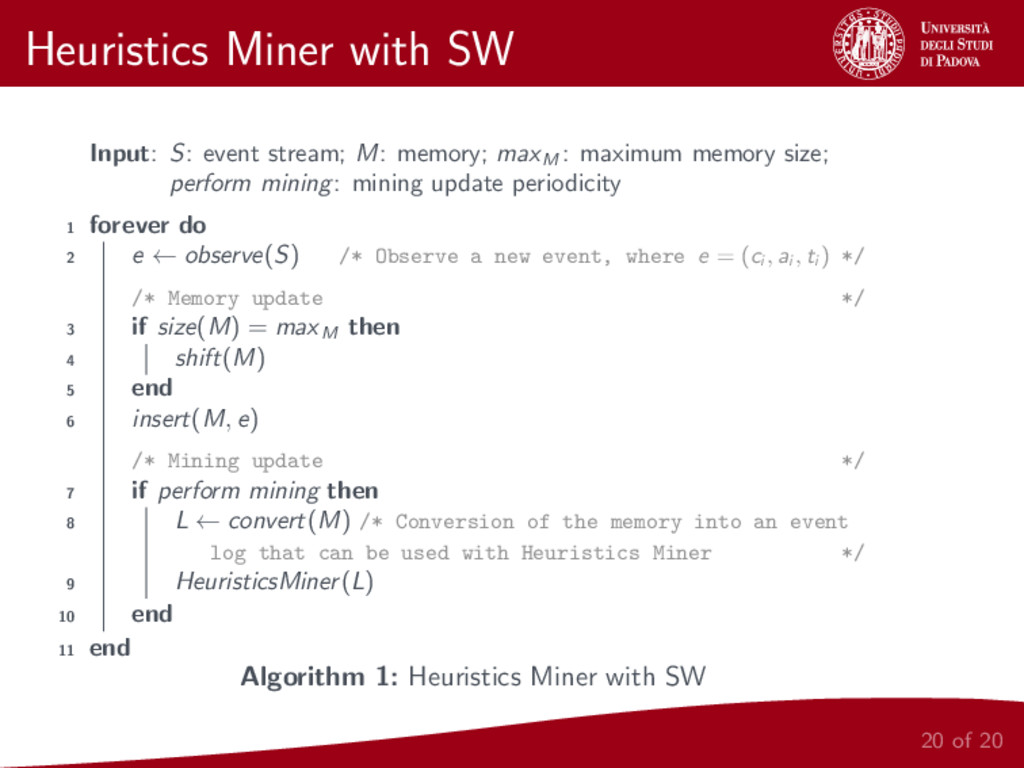
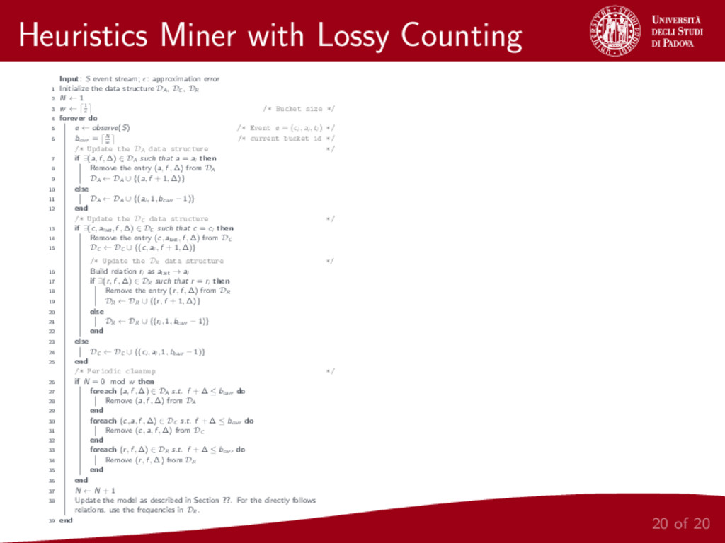
Two adaptations, based on Lossy Counting and Lossy Counting with Budget, as well as a sliding window based version of Heuristics Miner, are proposed and experimentally compared against both artificial and real streams. Experimental results show the effectiveness of control-flow discovery algorithms for streams on artificial and real datasets.

More info: http://andrea.burattin.net/publications/2014-cec

Transcript

1. Control-flow Discovery from Event Streams Andrea Burattin1, Alessandro Sperduti1, Wil M. P. van der Aalst2 1 University of Padua, Italy 2 Eindhoven University of Technology, The Netherlands July 11, 2014
2. Typical Process Mining Scenario Imagination Process Mining Incarnation / Environment Observation Operational Model Analytical Model Event Logs Information System Operational Incarnation support protocol / audit Discovery Conformance Extension control augment compare compare analyze mine basis create (re-)design implement describe Image source: Christian G¨ unther. Process mining in Flexible Environments, PhD thesis, Technische Universiteit Eindhoven, Eindhoven, 2009. 2 of 20
3. Typical Event Log Event # Activity Orig. Time . . . Case Id: C1 1 A U1 2014-01-01 . . . 2 B U1 2014-01-02 . . . 3 C U2 2014-01-03 . . . 4 E U2 2014-01-04 . . . Case Id: C2 1 A U1 2014-01-02 . . . 2 B U1 2014-01-03 . . . 3 D U3 2014-01-04 . . . 4 E U3 2014-01-05 . . . 3 of 20
4. Typical Event Log Event # Activity Orig. Time . . . Case Id: C1 1 A U1 2014-01-01 . . . 2 B U1 2014-01-02 . . . 3 C U2 2014-01-03 . . . 4 E U2 2014-01-04 . . . Case Id: C2 1 A U1 2014-01-02 . . . 2 B U1 2014-01-03 . . . 3 D U3 2014-01-04 . . . 4 E U3 2014-01-05 . . . Event # Case Id Activity Orig. Time . . . 1 C1 A U1 2014-01-01 . . . 2 C2 A U1 2014-01-02 . . . 3 C1 B U1 2014-01-02 . . . 4 C2 B U1 2014-01-03 . . . 5 C1 C U2 2014-01-03 . . . 6 C1 E U2 2014-01-04 . . . 7 C2 D U3 2014-01-04 . . . 8 C2 E U3 2014-01-05 . . . 3 of 20
5. Event Stream Representation of an event stream σ: E F E G F E F G G H I H H E F E G F E F G G H I H H σ Time Case: Cx Case: Cy Case: Cz Boxes represent events Background colors represent the case id Letters inside are the activity names 4 of 20
6. Streaming Process Discovery Events emi�ed over �me Stream miner instance ... Network communica�on Time ... A B B2 C A B C The stream miner continuously receives events and, using the latest observations, updates the process model (e.g., a Petri Net) 5 of 20
7. Stream Mining Peculiarities Peculiarities of the stream mining problem 6 of 20
8. Stream Mining Peculiarities Peculiarities of the stream mining problem 1 Cannot store the entire stream (approximation) 6 of 20
9. Stream Mining Peculiarities Peculiarities of the stream mining problem 1 Cannot store the entire stream (approximation) 2 Backtracking not feasible over streams (algorithms required to make one pass over data → scale linearly w.r.t. the number of processed items) 6 of 20
10. Stream Mining Peculiarities Peculiarities of the stream mining problem 1 Cannot store the entire stream (approximation) 2 Backtracking not feasible over streams (algorithms required to make one pass over data → scale linearly w.r.t. the number of processed items) 3 The approach must deal with variable system conditions, such as fluctuating stream rates 6 of 20
11. Stream Mining Peculiarities Peculiarities of the stream mining problem 1 Cannot store the entire stream (approximation) 2 Backtracking not feasible over streams (algorithms required to make one pass over data → scale linearly w.r.t. the number of processed items) 3 The approach must deal with variable system conditions, such as fluctuating stream rates 4 It is important to quickly adapt the model to cope with unusual data values (concept drifts) 6 of 20
12. Heuristics Miner Historical Background Our approaches are based on Heuristics Miner, quite old (∼ 2003) but still one of the most used algorithm 7 of 20
13. Heuristics Miner Historical Background Our approaches are based on Heuristics Miner, quite old (∼ 2003) but still one of the most used algorithm Fundamental metric is “dependency measure” between two activities (e.g. a, b): a ⇒ b = |a > b| − |b > a| |a > b| + |b > a| + 1 ∈ [−1, 1] Where: |a > b| is the number of times that a > b holds in the log a > b holds if a executed at time t and b at t + 1 7 of 20
14. Heuristics Miner (cont.) Given the dependency measure for all activity pairs and a threshold τdep, the algorithm builds a directed dependency graph 8 of 20
15. Heuristics Miner (cont.) Given the dependency measure for all activity pairs and a threshold τdep, the algorithm builds a directed dependency graph If both a ⇒ b > τdep and a ⇒ c > τdep then: a b c Relation ambiguity between b and c: XOR: either b or c is executed AND: both b and c are executed 8 of 20
16. Heuristics Miner (cont.) Given the dependency measure for all activity pairs and a threshold τdep, the algorithm builds a directed dependency graph If both a ⇒ b > τdep and a ⇒ c > τdep then: a b c Relation ambiguity between b and c: XOR: either b or c is executed AND: both b and c are executed Heuristics Miner proposes the “AND-measure” a ⇒ (b ∧ c) = |b > c| + |c > b| |a > b| + |a > c| + 1 ∈ [0, 1] If a ⇒ (b ∧ c) > τand then AND relation, XOR otherwise 8 of 20
17. Direct Following Matrix Basic data structure for HM is Direct Following Matrix Direct Following Matrix Given activities A, B, C, D and a log L, |a > b| is the number of times that a is directly followed by b (within the same process instance) in the log L A B C D A 0 52 64 91 B 52 0 24 87 C 64 24 0 13 D 91 87 13 0 9 of 20
18. Proposed Approaches Our Proposal We present three approaches, based on Heuristics Miner, for process discovery from event streams: (SW) Heuristics Miner with Sliding Window (as baseline) (LC) Heuristics Miner with Lossy Counting (LCB) Heuristics Miner with Lossy Counting with Budget 10 of 20
19. Proposed Approaches Our Proposal We present three approaches, based on Heuristics Miner, for process discovery from event streams: (SW) Heuristics Miner with Sliding Window (as baseline) (LC) Heuristics Miner with Lossy Counting (LCB) Heuristics Miner with Lossy Counting with Budget Fundamental Principle Recent observations are more important than older ones 10 of 20
20. Heuristics Miner with SW Basic idea is to iterate these steps 1 Collect events for a given time span 2 Generate a finite event log 3 Apply the “offline version” of the algorithm { Time frame considered Mining �me Log used for mining 11 of 20
21. Frequency Counting with Lossy Counting Given Max approximation error Variables: A , B , C Bucket size is w = 1 bcurrent = no. of observed items w Lossy Counting uses a data structure D = {(var, freq, max error)} 12 of 20
22. Frequency Counting with Lossy Counting Given Max approximation error Variables: A , B , C Bucket size is w = 1 bcurrent = no. of observed items w Lossy Counting uses a data structure D = {(var, freq, max error)} A A B A B C C B C A A B C Data sequence Buckets If B not present then (B, f = 1, Δ = bcurrent ‐ 1) else Update frequency f of B bcurrent Remove all elements s.t. f + Δ ≤ bcurrent bcurrent + 1 12 of 20
23. LC/LCB Demo Lossy Counting Demo f Δ → 0 0 0 0 0 f 0 0 ← Δ Time Remove if f + Δ ≤ 1 bcurrent = 1 End of bucket 1 Beginning of bucket 2 13 of 20
24. LC/LCB Demo Lossy Counting Demo f 0 0 ← Δ Time Beginning of bucket 2 f Δ → 0 0 1 1 f 0 0 1 ← Δ Remove if f + Δ ≤ 2 bcurrent = 2 End of bucket 2 Beginning of bucket 3 13 of 20
25. LC/LCB Demo Lossy Counting Demo Time f 0 0 1 ← Δ Beginning of bucket 3 f Δ → 0 0 1 2 f 0 0 1 2 ← Δ Remove if f + Δ ≤ 3 bcurrent = 3 End of bucket 3 Beginning of bucket 4 13 of 20
26. LC/LCB Demo Comparison between Lossy Counting frequencies and true frequencies f F Δ → 0 0 1 2 Es�mated frequencies True frequencies These inequalities hold: f ≤ F ≤ f + ∆ ≤ f + N 13 of 20
27. LC/LCB Demo Comparison between Lossy Counting frequencies and true frequencies f F Δ → 0 0 1 2 Es�mated frequencies True frequencies These inequalities hold: f ≤ F ≤ f + ∆ ≤ f + N Lossy Counting with Budget Idea New bucket when there is no more space, then = 1 bucket size 13 of 20
28. Adaptation of LC/LCB to HM To count direct following relations we need Drel Actual relations frequencies, tuples: (as, at, f , ∆) Dact Latest activity names, tuples: (a, f , ∆) Dcases Latest activity of a case, tuples: (c, a, f , ∆) 14 of 20
29. Adaptation of LC/LCB to HM To count direct following relations we need Drel Actual relations frequencies, tuples: (as, at, f , ∆) Dact Latest activity names, tuples: (a, f , ∆) Dcases Latest activity of a case, tuples: (c, a, f , ∆) With a certain periodicity, model update Activities from Dact Dependencies and AND/XOR rules from Drel 14 of 20
30. Adaptation of LC/LCB to HM To count direct following relations we need Drel Actual relations frequencies, tuples: (as, at, f , ∆) Dact Latest activity names, tuples: (a, f , ∆) Dcases Latest activity of a case, tuples: (c, a, f , ∆) With a certain periodicity, model update Activities from Dact Dependencies and AND/XOR rules from Drel Actually, we show that updates on D data structures affect only local parts of the model (incremental update of the process model) 14 of 20
31. Evaluation Datasets Artificial dataset characteristics: Three randomly generated processes (to simulate concept drifts) Most complex model has 3 splits (1 AND and 2 XOR) Longest process has 16 activities Stream with 17 265 events Real-world dataset (BPI Challenge 2012 log) characteristics Dutch Financial Institute 36 activities 262 198 events, among 13 087 process instances 15 of 20
32. Evaluation on Artificial Dataset Model-to-model Metric Assess the correspondence between original and discovered model 0 0.1 0.2 0.3 0.4 0.5 0.6 0.7 0.8 0.9 1 0 2000 4000 6000 8000 10000 12000 14000 16000 18000 Model‐to‐model similarity Observed events LCB (B = 300) LCB (B = 100) LC (ε = 0.000001) LC (ε = 0.001) SW (W = 300) SW (W = 100) 16 of 20
33. Evaluation on Artificial Dataset Space Requirements Space expressed as number of stored items 0 250 500 750 1000 1250 1500 1750 2000 0 2000 4000 6000 8000 10000 12000 14000 16000 18000 No. stored items Observed events LCB (B = 300) LCB (B = 100) LC (ε = 0.000001) LC (ε = 0.001) SW (W = 300) SW (W = 100) 17 of 20
34. Evaluation on Artificial Dataset Time Requirements Time required to process each event 0 5 10 15 20 0 2000 4000 6000 8000 10000 12000 14000 16000 18000 Time per event (ms) Observed events LCB (B = 300) LCB (B = 100) LC (ε = 0.000001) LC (ε = 0.001) SW (W = 300) SW (W = 100) 18 of 20
35. Evaluation on BPI Challenge 2012 Precision Metric Precision of the discovered models 0 0.2 0.4 0.6 0.8 1 0*100 50*103 100*103 150*103 200*103 250*103 Precision Observed events SW (W = 1000) LC (ε = 0.00001) LCB (B = 1000) Time required to process an event: SW: 24.59ms LC: 5.68ms LCB: 2.56ms 19 of 20
36. Conclusions and Future Work Conclusions We addressed the problem of discovering process models from event streams Three approaches proposed, based on Heuristics Miner (with Sliding Window, with Lossy Counting, and with Lossy Counting with Budget) Experimental results on both artificial and real dataset, with improvements in terms of quality of the mined models, execution time, and space requirements as well Future Work Improve the process analyst to mine different perspectives Animations to point out process drifts locations 20 of 20
37. End. 20 of 20
38. Heuristics Miner with SW Input: S: event stream; M: memory; maxM : maximum memory size; perform mining: mining update periodicity 1 forever do 2 e ← observe(S) /* Observe a new event, where e = (ci , ai , ti ) */ /* Memory update */ 3 if size(M) = maxM then 4 shift(M) 5 end 6 insert(M, e) /* Mining update */ 7 if perform mining then 8 L ← convert(M) /* Conversion of the memory into an event log that can be used with Heuristics Miner */ 9 HeuristicsMiner(L) 10 end 11 end Algorithm 1: Heuristics Miner with SW 20 of 20
39. Heuristics Miner with Lossy Counting Input: S event stream; : approximation error 1 Initialize the data structure DA , DC , DR 2 N ← 1 3 w ← 1 /* Bucket size */ 4 forever do 5 e ← observe(S) /* Event e = (ci , ai , ti ) */ 6 bcurr = N w /* current bucket id */ /* Update the DA data structure */ 7 if ∃(a, f , ∆) ∈ DA such that a = ai then 8 Remove the entry (a, f , ∆) from DA 9 DA ← DA ∪ {(a, f + 1, ∆)} 10 else 11 DA ← DA ∪ {(ai , 1, bcurr − 1)} 12 end /* Update the DC data structure */ 13 if ∃(c, alast , f , ∆) ∈ DC such that c = ci then 14 Remove the entry (c, alast , f , ∆) from DC 15 DC ← DC ∪ {(c, ai , f + 1, ∆)} /* Update the DR data structure */ 16 Build relation ri as alast → ai 17 if ∃(r, f , ∆) ∈ DR such that r = ri then 18 Remove the entry (r, f , ∆) from DR 19 DR ← DR ∪ {(r, f + 1, ∆)} 20 else 21 DR ← DR ∪ {(ri , 1, bcurr − 1)} 22 end 23 else 24 DC ← DC ∪ {(ci , ai , 1, bcurr − 1)} 25 end /* Periodic cleanup */ 26 if N = 0 mod w then 27 foreach (a, f , ∆) ∈ DA s.t. f + ∆ ≤ bcurr do 28 Remove (a, f , ∆) from DA 29 end 30 foreach (c, a, f , ∆) ∈ DC s.t. f + ∆ ≤ bcurr do 31 Remove (c, a, f , ∆) from DC 32 end 33 foreach (r, f , ∆) ∈ DR s.t. f + ∆ ≤ bcurr do 34 Remove (r, f , ∆) from DR 35 end 36 end 37 N ← N + 1 38 Update the model as described in Section ??. For the directly follows relations, use the frequencies in DR . 39 end 20 of 20
40. Evaluation on BPI Challenge 2012 Precision vs Fitness Metric Precision (SW) 250500 1000 2000 Evalua�on log sizes 250 500 1000 2000 Window size 0.5 0.55 0.6 0.65 0.7 0.75 0.8 0.85 Fitness (SW) 250500 1000 2000 Evalua�on log sizes 250 500 1000 2000 0.62 0.64 0.66 0.68 0.7 0.72 0.74 0.76 0.78 Precision (LCB) 250500 1000 2000 Evalua�on log sizes 250 500 1000 2000 Budget 0.74 0.76 0.78 0.8 0.82 0.84 0.86 Fitness (LCB) 250500 1000 2000 Evalua�on log sizes 250 500 1000 2000 0.4 0.41 0.42 0.43 0.44 0.45 0.46 0.47 0.48 0.49 0.5 0.51 Precision (LC) 250500 1000 2000 Evalua�on log sizes 1e‐05 0.001 0.1 ε 0.75 0.8 0.85 0.9 0.95 1 Fitness (LC) 250500 1000 2000 Evalua�on log sizes 1e‐05 0.001 0.1 0.4 0.42 0.44 0.46 0.48 0.5 0.52 0.54 0.56 0.58 20 of 20
41. Evaluation on Artificial Dataset Space Distribution over Data Structures Space required by LCB (with B = 300) to store activities (DA), relations (DR) and cases (DC ) 0 50 100 150 200 250 300 0 2000 4000 6000 8000 10000 12000 14000 16000 No. sotred item Observed events Size of DA Size of DR Size of DC 20 of 20