Online Conformance Checking Using Behavioural Patterns

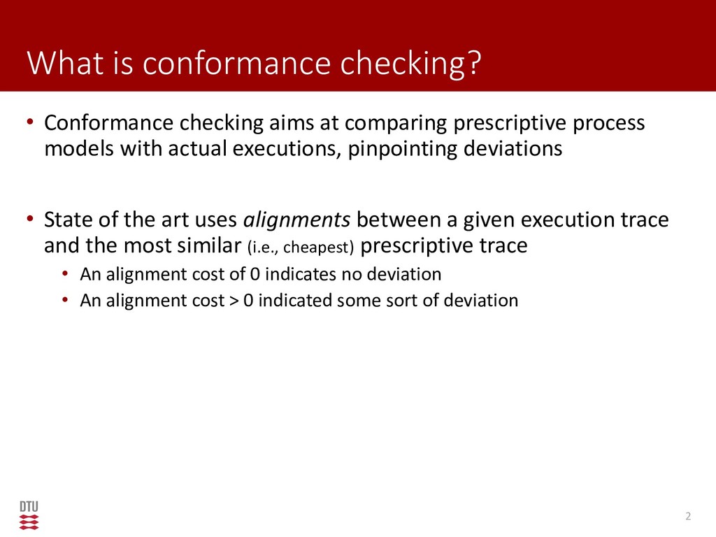
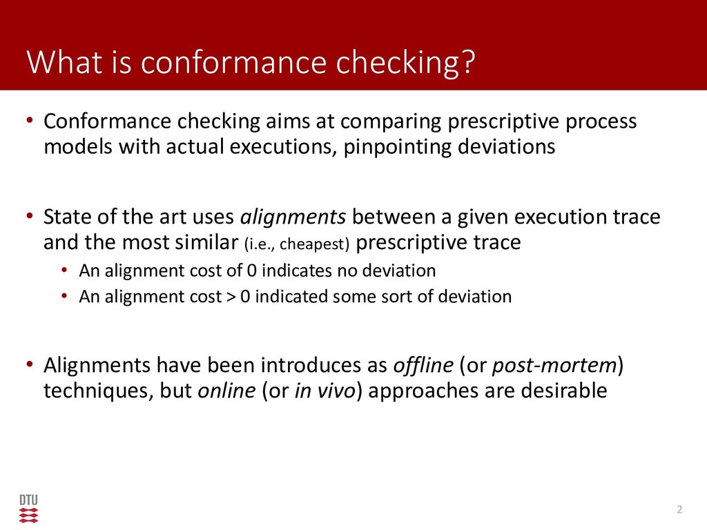
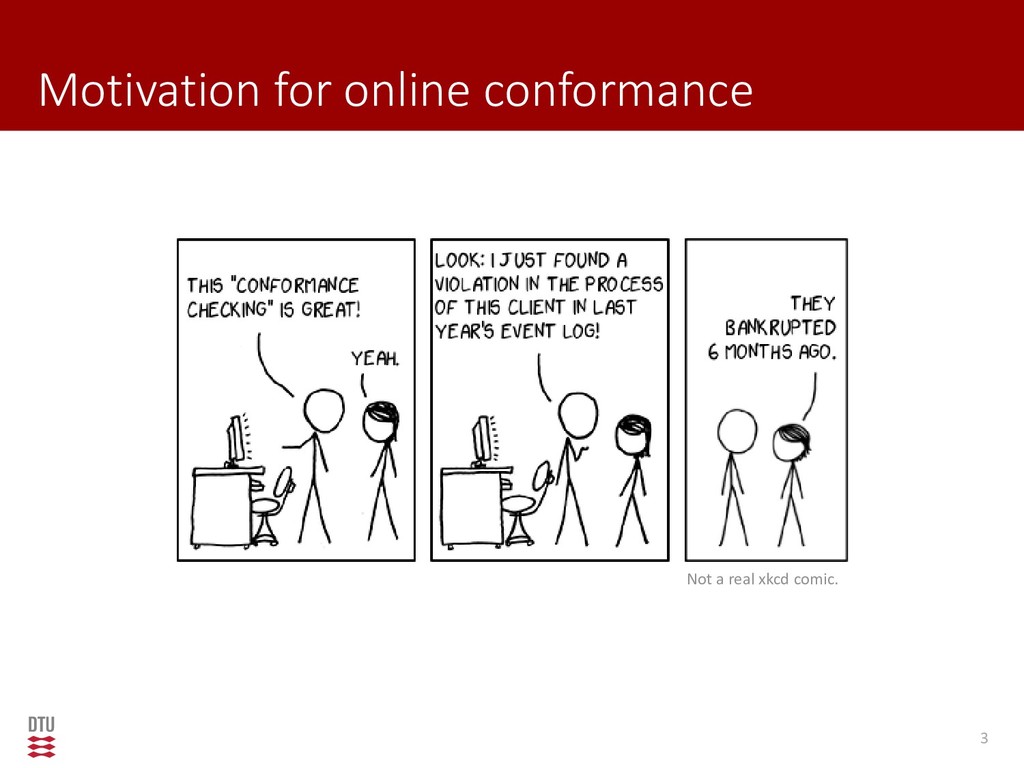
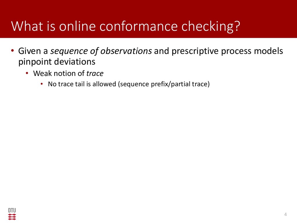
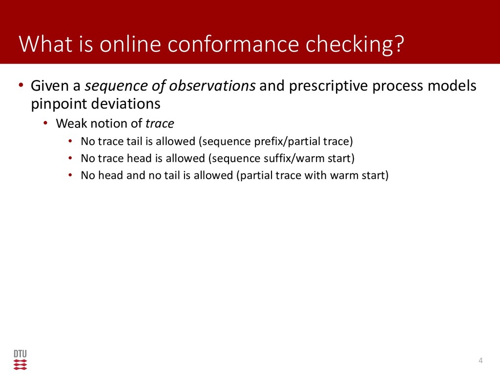
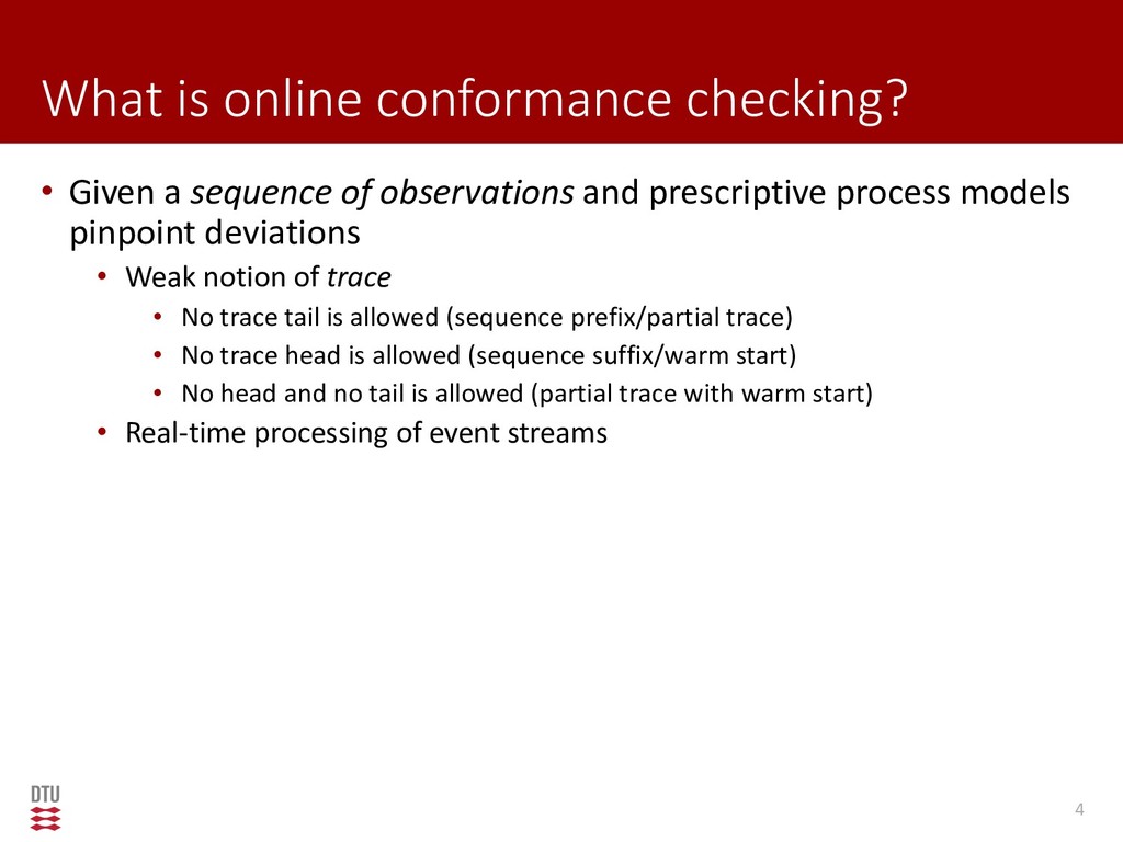
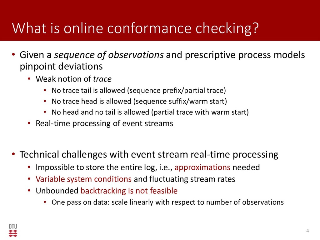
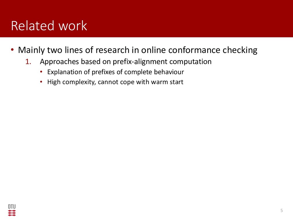
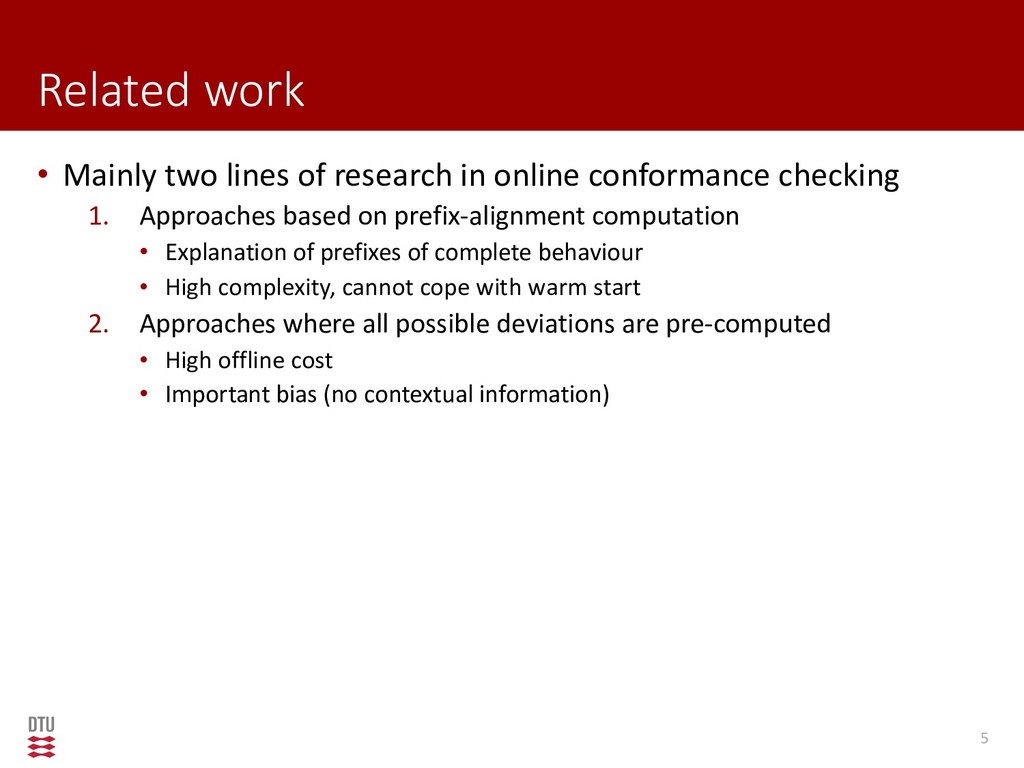
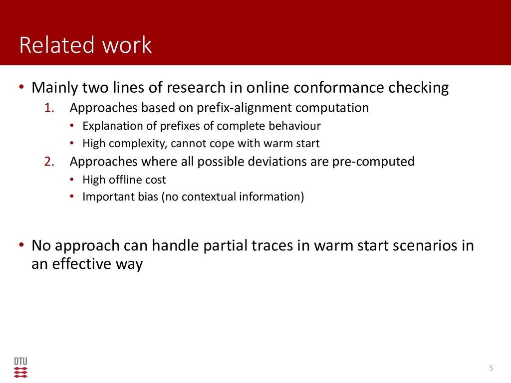
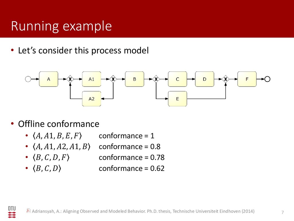
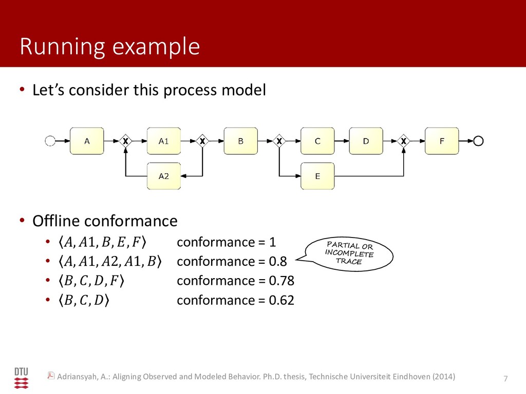
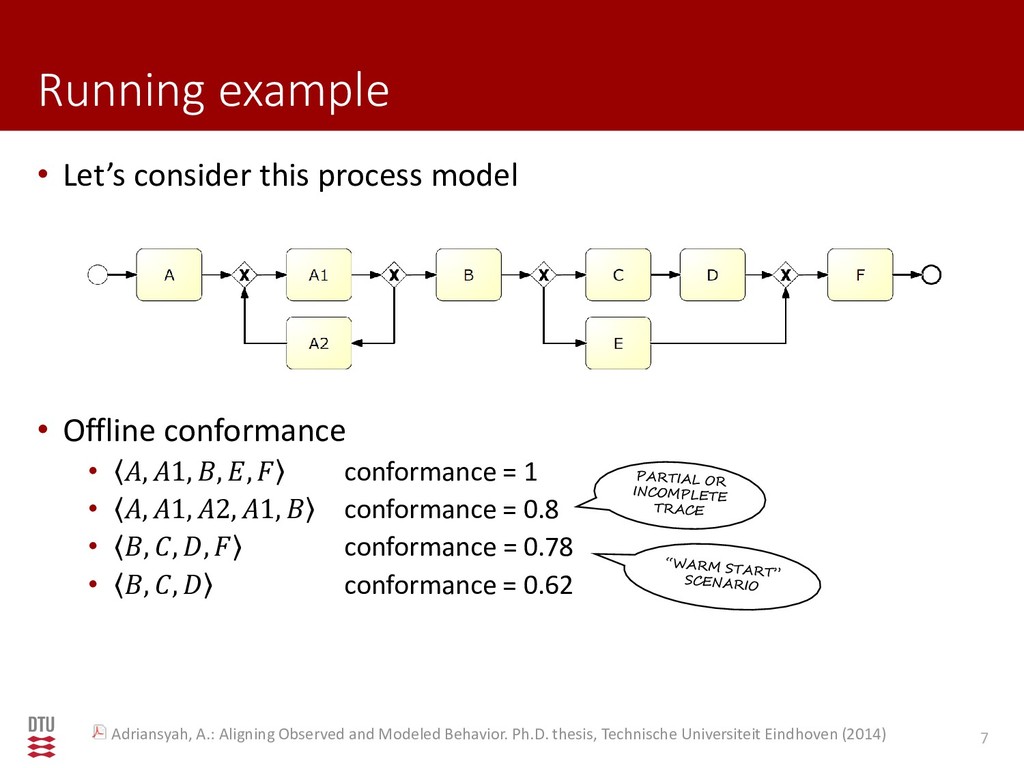
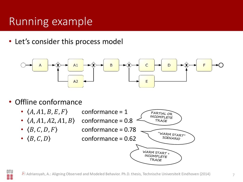
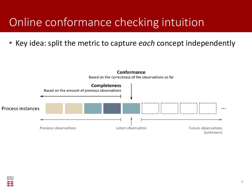
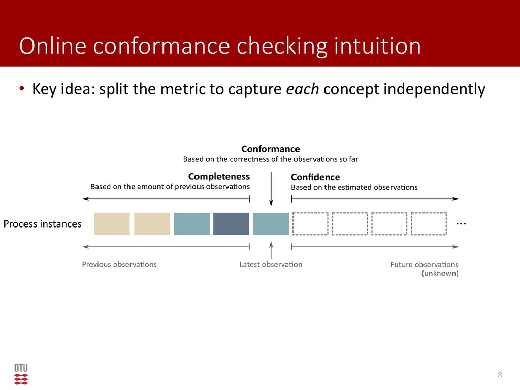
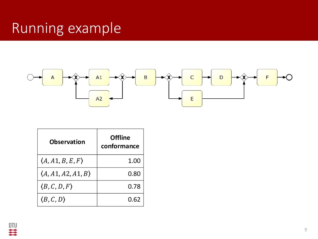
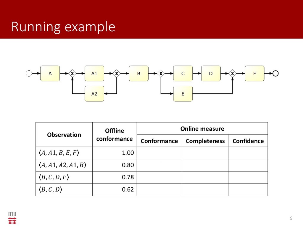
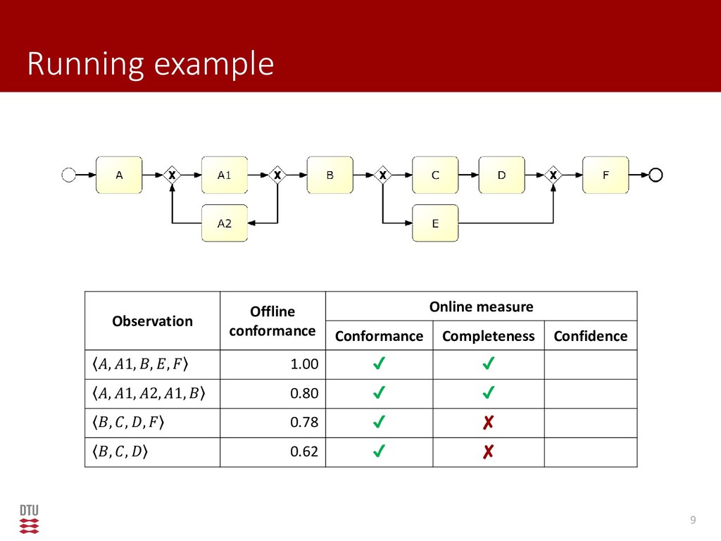
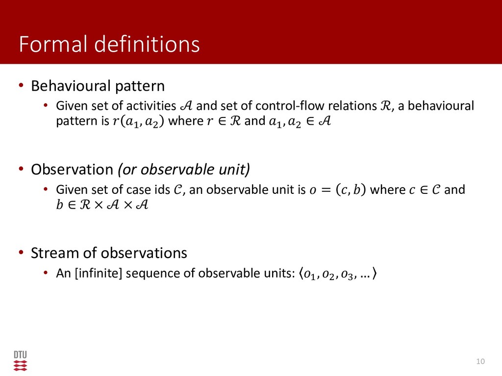
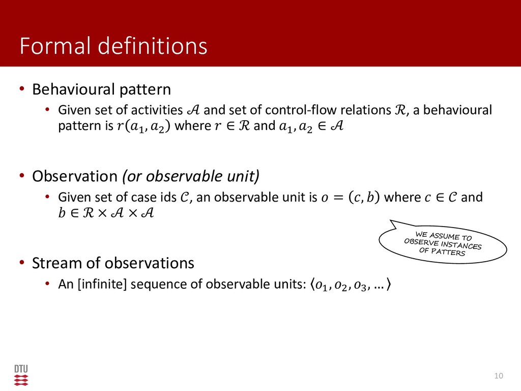
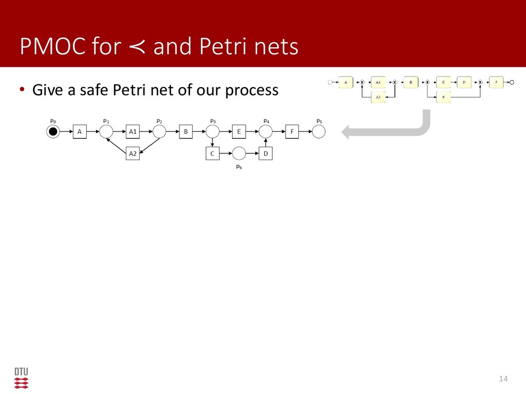
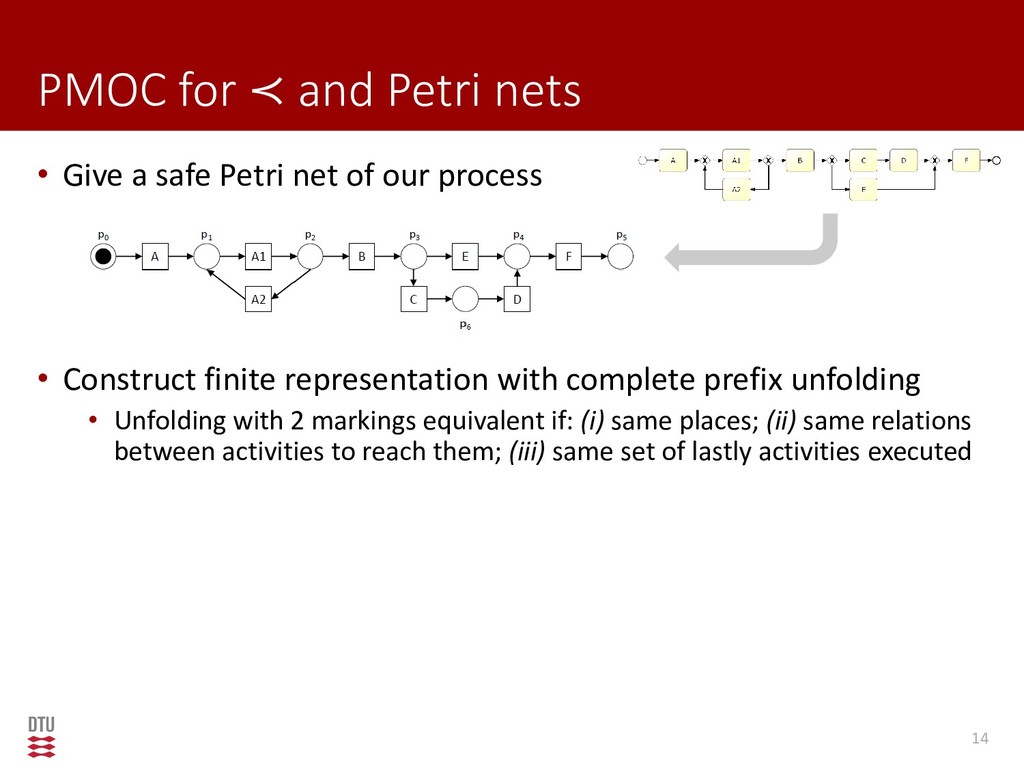
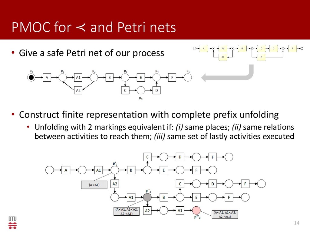
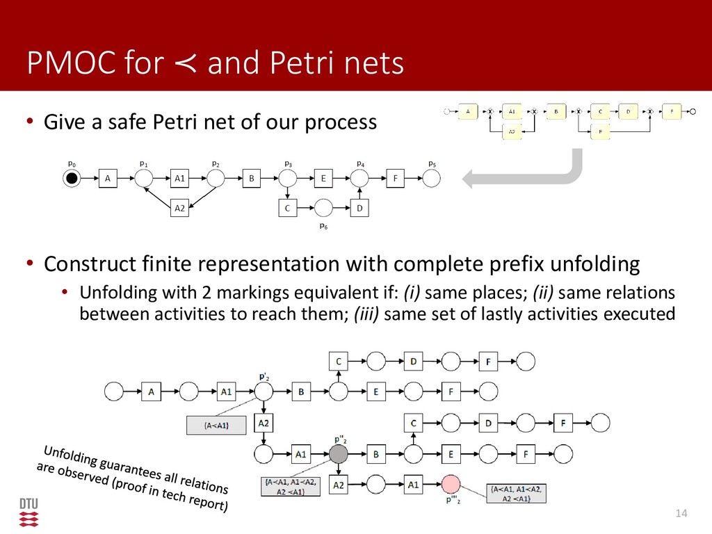
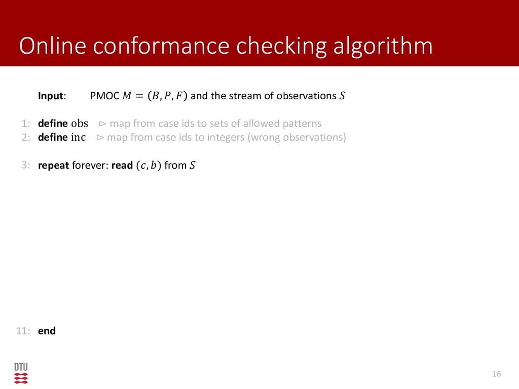
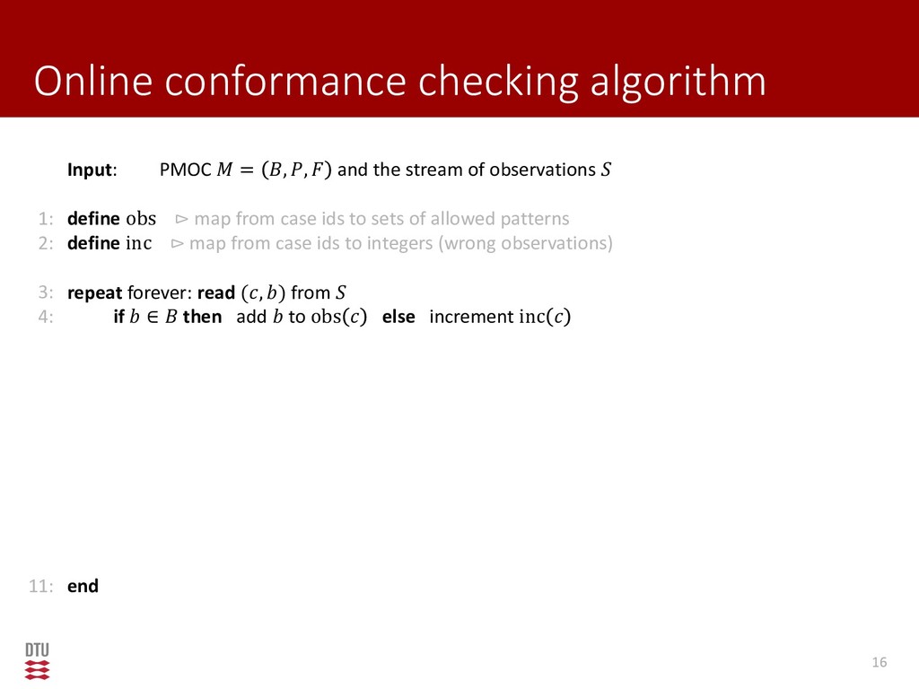
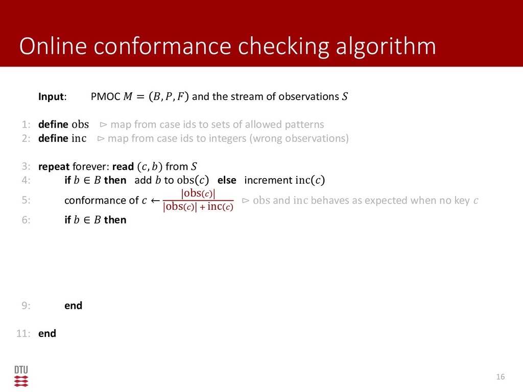
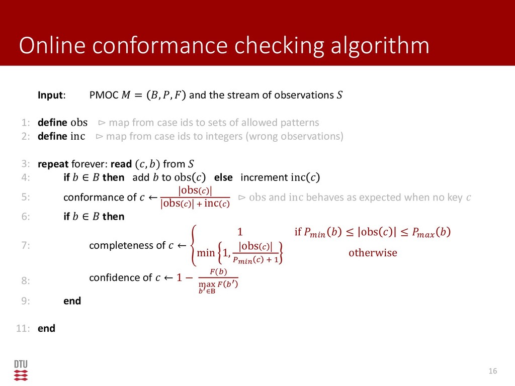
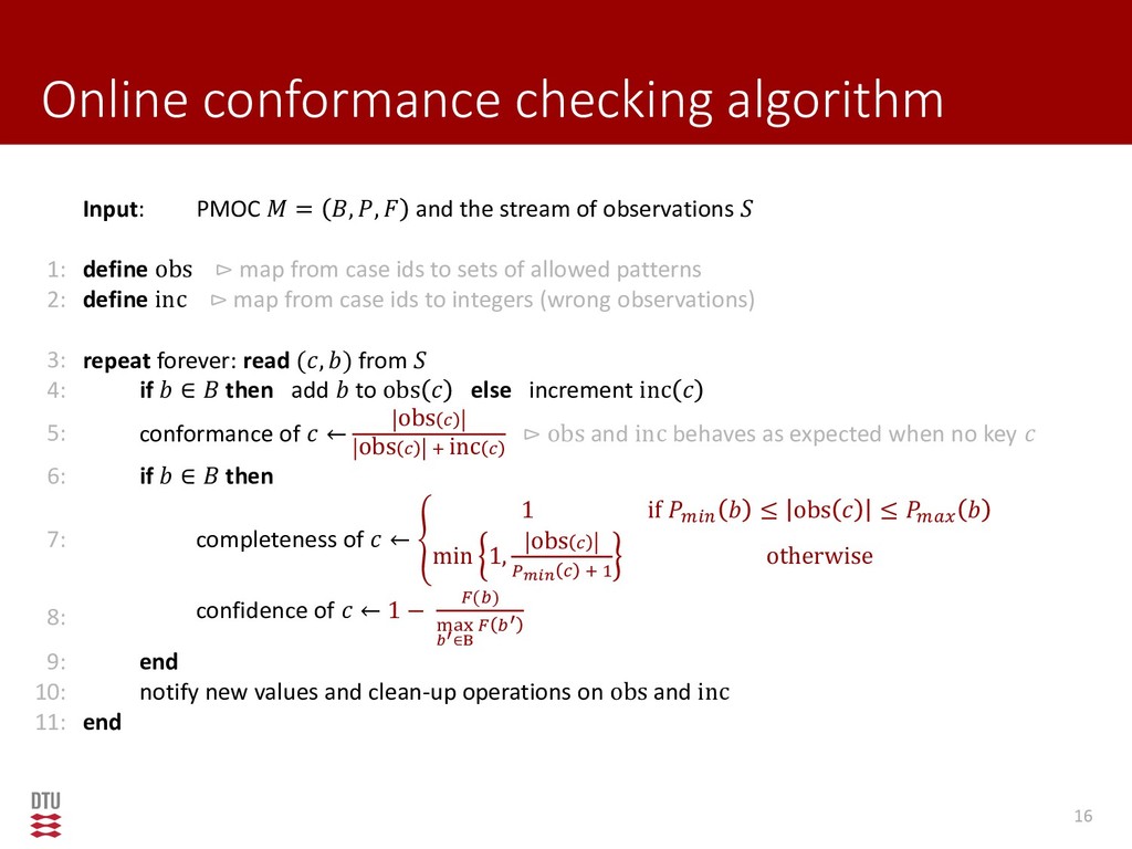
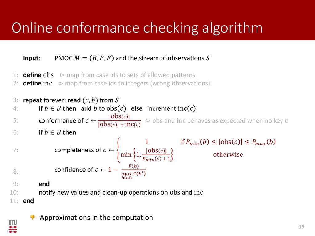
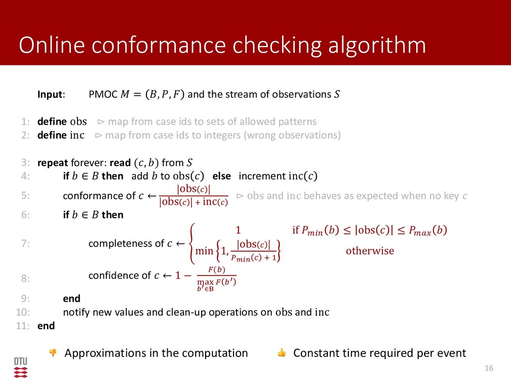
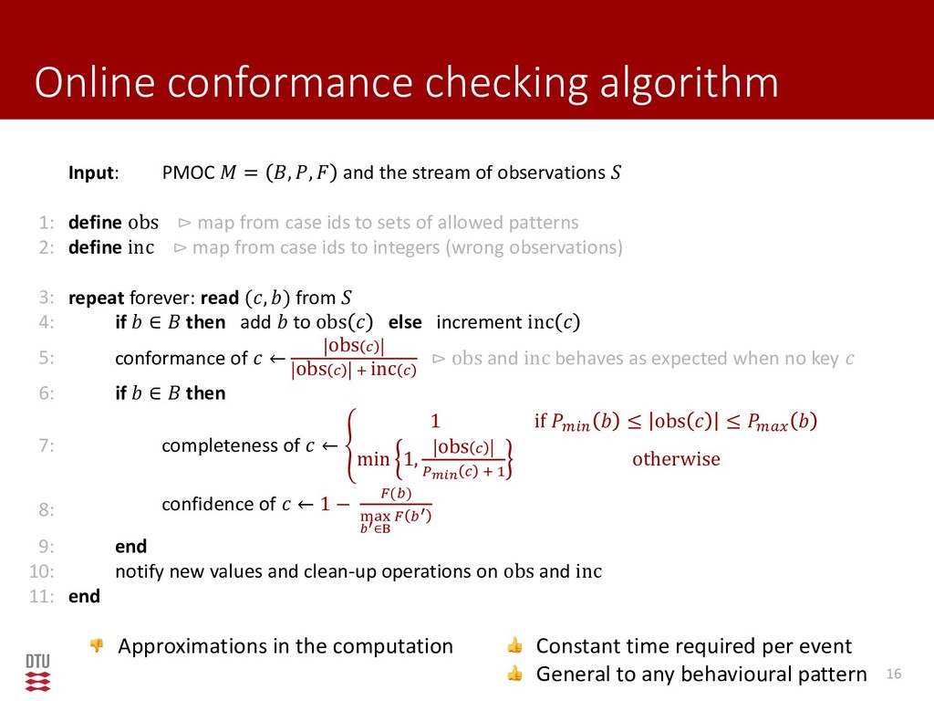
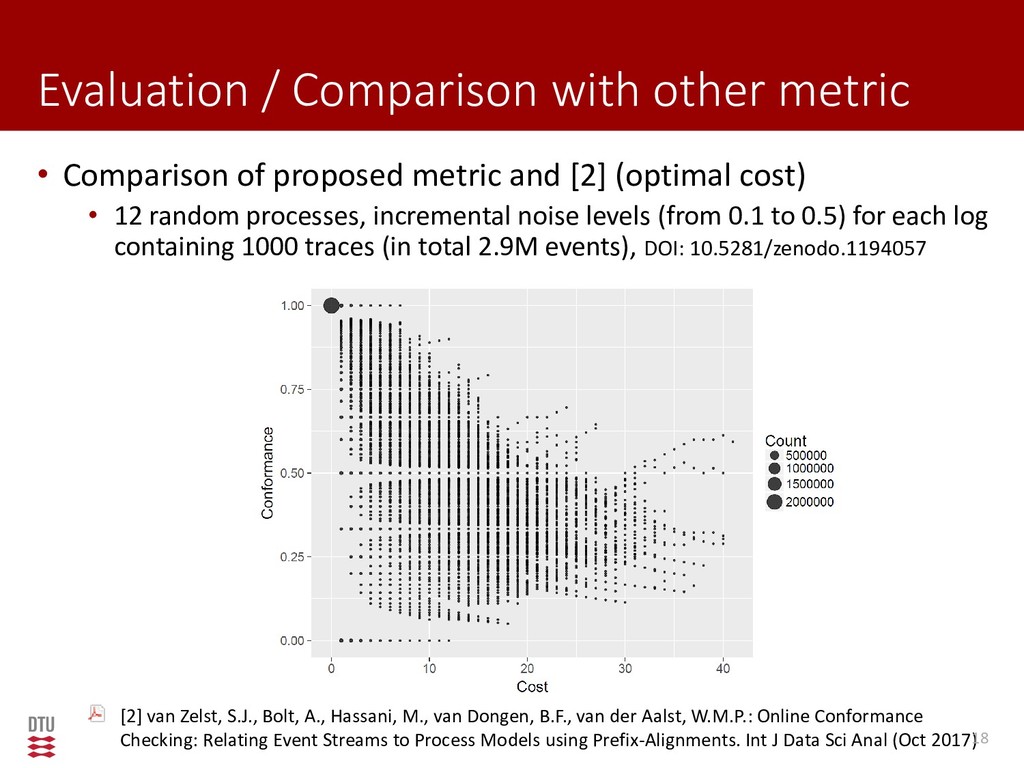
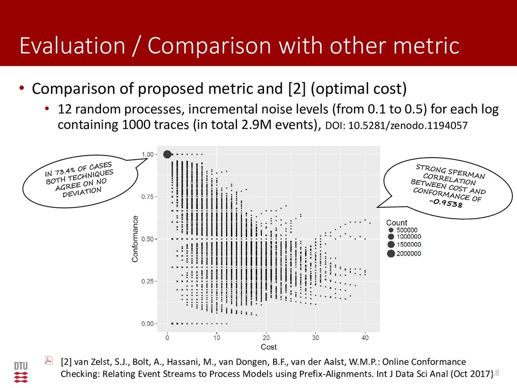
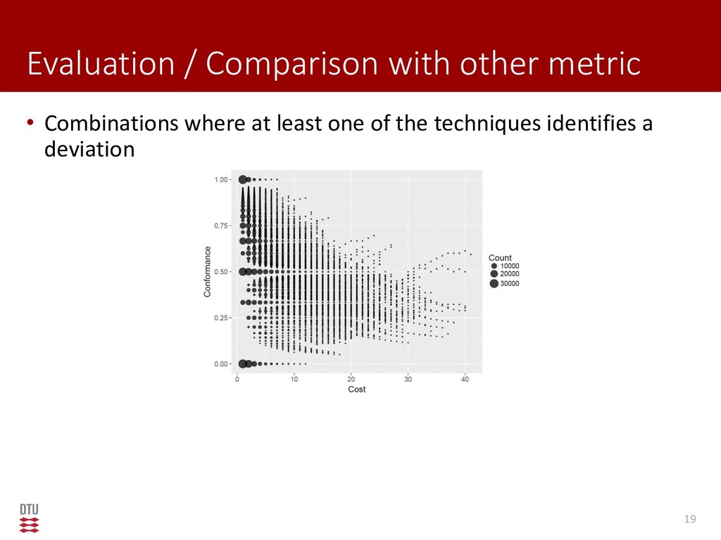
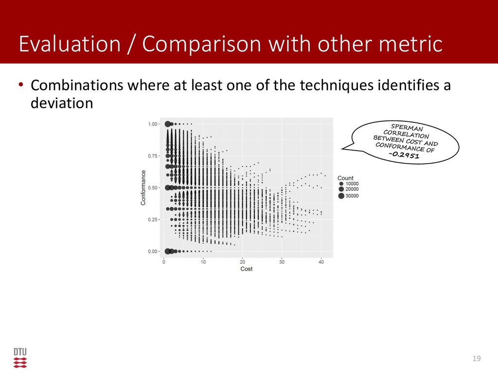
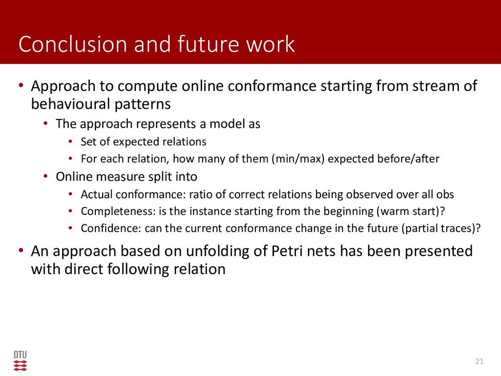
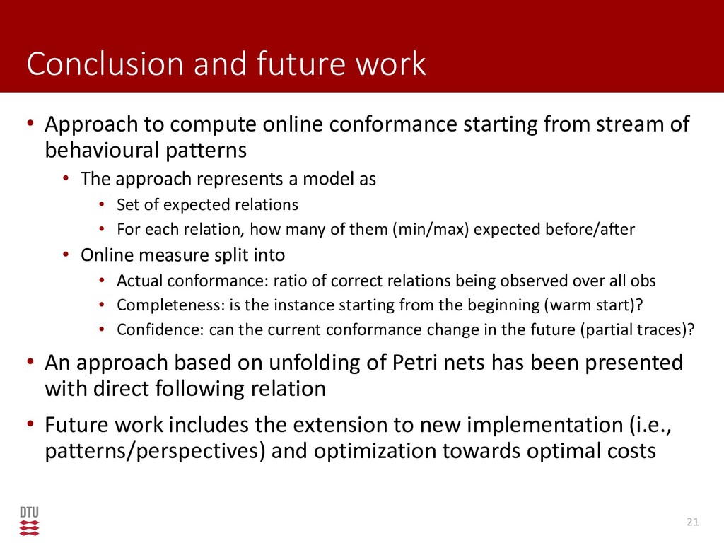
New and compelling regulations (e.g., the GDPR in Europe) impose tremendous pressure on organizations, in order to adhere to standard procedures, processes, and practices. The field of conformance checking aims to quantify the extent to which the execution of a process, captured within recorded corresponding event data, conforms to a given reference process model. Existing techniques assume a post-mortem scenario, i.e. they detect deviations based on complete executions of the process. This limits their applicability in an online setting. In such context, we aim to to detect deviations online (i.e., in-vivo), in order to provide recovery possibilities before the execution of a process instance is completed. Also, current techniques assume cases to start from the initial stage of the process, whereas this assumption is not feasible in online settings. In this paper, we present a generic framework for online conformance checking, in which the underlying process is represented in terms of behavioural patterns and no assumption on the starting point of cases is needed. We instantiate the framework on the basis of Petri nets, with an accompanying new unfolding technique. The approach is implemented in the process mining tool ProM, and evaluated by means of several experiments including a stress-test and a comparison with a similar technique.

More info: https://andrea.burattin.net/publications/2018-bpm

Transcript

1. Online Conformance Checking Using Behavioural Patterns A. Burattin1, S. van Zelst 2, A. Armas-Cervantes3, B. van Dongen 2, J. Carmona 4 1 Technical University of Denmark, Kgs. Lyngby, Denmark 2 Eindhoven University of Technology, Eindhoven, The Netherlands 3 The University of Melbourne, Melbourne, Australia 4 Universitat Politècnica de Catalunya, Barcelona, Spain
2. What is conformance checking? • Conformance checking aims at comparing prescriptive process models with actual executions, pinpointing deviations 2
3. What is conformance checking? • Conformance checking aims at comparing prescriptive process models with actual executions, pinpointing deviations • State of the art uses alignments between a given execution trace and the most similar (i.e., cheapest) prescriptive trace • An alignment cost of 0 indicates no deviation • An alignment cost > 0 indicated some sort of deviation 2
4. What is conformance checking? • Conformance checking aims at comparing prescriptive process models with actual executions, pinpointing deviations • State of the art uses alignments between a given execution trace and the most similar (i.e., cheapest) prescriptive trace • An alignment cost of 0 indicates no deviation • An alignment cost > 0 indicated some sort of deviation • Alignments have been introduces as offline (or post-mortem) techniques, but online (or in vivo) approaches are desirable 2
5. Motivation for online conformance Not a real xkcd comic. 3
6. What is online conformance checking? • Given a sequence of observations and prescriptive process models pinpoint deviations • Weak notion of trace 4
7. What is online conformance checking? • Given a sequence of observations and prescriptive process models pinpoint deviations • Weak notion of trace • No trace tail is allowed (sequence prefix/partial trace) 4
8. What is online conformance checking? • Given a sequence of observations and prescriptive process models pinpoint deviations • Weak notion of trace • No trace tail is allowed (sequence prefix/partial trace) • No trace head is allowed (sequence suffix/warm start) 4
9. What is online conformance checking? • Given a sequence of observations and prescriptive process models pinpoint deviations • Weak notion of trace • No trace tail is allowed (sequence prefix/partial trace) • No trace head is allowed (sequence suffix/warm start) • No head and no tail is allowed (partial trace with warm start) 4
10. What is online conformance checking? • Given a sequence of observations and prescriptive process models pinpoint deviations • Weak notion of trace • No trace tail is allowed (sequence prefix/partial trace) • No trace head is allowed (sequence suffix/warm start) • No head and no tail is allowed (partial trace with warm start) • Real-time processing of event streams 4
11. What is online conformance checking? • Given a sequence of observations and prescriptive process models pinpoint deviations • Weak notion of trace • No trace tail is allowed (sequence prefix/partial trace) • No trace head is allowed (sequence suffix/warm start) • No head and no tail is allowed (partial trace with warm start) • Real-time processing of event streams • Technical challenges with event stream real-time processing • Impossible to store the entire log, i.e., approximations needed • Variable system conditions and fluctuating stream rates • Unbounded backtracking is not feasible • One pass on data: scale linearly with respect to number of observations 4
12. Related work • Mainly two lines of research in online conformance checking 5
13. Related work • Mainly two lines of research in online conformance checking 1. Approaches based on prefix-alignment computation • Explanation of prefixes of complete behaviour • High complexity, cannot cope with warm start 5
14. Related work • Mainly two lines of research in online conformance checking 1. Approaches based on prefix-alignment computation • Explanation of prefixes of complete behaviour • High complexity, cannot cope with warm start 2. Approaches where all possible deviations are pre-computed • High offline cost • Important bias (no contextual information) 5
15. Related work • Mainly two lines of research in online conformance checking 1. Approaches based on prefix-alignment computation • Explanation of prefixes of complete behaviour • High complexity, cannot cope with warm start 2. Approaches where all possible deviations are pre-computed • High offline cost • Important bias (no contextual information) • No approach can handle partial traces in warm start scenarios in an effective way 5
16. Table of contents • Introduction and motivation • Online conformance checking • Intuition • General approach for behavioural patterns • Instance to direct following relations • Experimental evaluation • Conclusion 6
17. Running example • Let’s consider this process model • Offline conformance • , 1, , , conformance = 1 • , 1, 2, 1, conformance = 0.8 • , , , conformance = 0.78 • , , conformance = 0.62 Adriansyah, A.: Aligning Observed and Modeled Behavior. Ph.D. thesis, Technische Universiteit Eindhoven (2014) 7
18. Running example • Let’s consider this process model • Offline conformance • , 1, , , conformance = 1 • , 1, 2, 1, conformance = 0.8 • , , , conformance = 0.78 • , , conformance = 0.62 Adriansyah, A.: Aligning Observed and Modeled Behavior. Ph.D. thesis, Technische Universiteit Eindhoven (2014) 7
19. Running example • Let’s consider this process model • Offline conformance • , 1, , , conformance = 1 • , 1, 2, 1, conformance = 0.8 • , , , conformance = 0.78 • , , conformance = 0.62 Adriansyah, A.: Aligning Observed and Modeled Behavior. Ph.D. thesis, Technische Universiteit Eindhoven (2014) 7
20. Running example • Let’s consider this process model • Offline conformance • , 1, , , conformance = 1 • , 1, 2, 1, conformance = 0.8 • , , , conformance = 0.78 • , , conformance = 0.62 Adriansyah, A.: Aligning Observed and Modeled Behavior. Ph.D. thesis, Technische Universiteit Eindhoven (2014) 7
21. Online conformance checking intuition • Key idea: split the metric to capture each concept independently 8
22. Online conformance checking intuition • Key idea: split the metric to capture each concept independently 8
23. Online conformance checking intuition • Key idea: split the metric to capture each concept independently 8
24. Online conformance checking intuition • Key idea: split the metric to capture each concept independently 8
25. Online conformance checking intuition • Key idea: split the metric to capture each concept independently 8
26. Online conformance checking intuition • Key idea: split the metric to capture each concept independently 8
27. Online conformance checking intuition • Key idea: split the metric to capture each concept independently 8
28. Running example Observation Offline conformance Online measure Conformance Completeness Confidence , 1, , , 1.00 ✔ ✔ High , 1, 2, 1, 0.80 ✔ ✔ Low , , , 0.78 ✔ ✘ High , , 0.62 ✔ ✘ Low 9
29. Running example Observation Offline conformance Online measure Conformance Completeness Confidence , 1, , , 1.00 ✔ ✔ High , 1, 2, 1, 0.80 ✔ ✔ Low , , , 0.78 ✔ ✘ High , , 0.62 ✔ ✘ Low 9
30. Running example Observation Offline conformance Online measure Conformance Completeness Confidence , 1, , , 1.00 ✔ ✔ High , 1, 2, 1, 0.80 ✔ ✔ Low , , , 0.78 ✔ ✘ High , , 0.62 ✔ ✘ Low 9
31. Running example Observation Offline conformance Online measure Conformance Completeness Confidence , 1, , , 1.00 ✔ ✔ High , 1, 2, 1, 0.80 ✔ ✔ Low , , , 0.78 ✔ ✘ High , , 0.62 ✔ ✘ Low 9
32. Running example Observation Offline conformance Online measure Conformance Completeness Confidence , 1, , , 1.00 ✔ ✔ High , 1, 2, 1, 0.80 ✔ ✔ Low , , , 0.78 ✔ ✘ High , , 0.62 ✔ ✘ Low 9
33. Formal definitions • Behavioural pattern • Given set of activities and set of control-flow relations ℛ, a behavioural pattern is 1 , 2 where ∈ ℛ and 1 , 2 ∈ • Observation (or observable unit) • Given set of case ids , an observable unit is = , where ∈ and ∈ ℛ × × • Stream of observations • An [infinite] sequence of observable units: 1 , 2 , 3 , … 10
34. Formal definitions • Behavioural pattern • Given set of activities and set of control-flow relations ℛ, a behavioural pattern is 1 , 2 where ∈ ℛ and 1 , 2 ∈ • Observation (or observable unit) • Given set of case ids , an observable unit is = , where ∈ and ∈ ℛ × × • Stream of observations • An [infinite] sequence of observable units: 1 , 2 , 3 , … 10
35. Pattern instances as observations • A stream of behavioural patterns represents high level information • To obtain such stream, pre-processing might be required • For many control-flow relations, approaches already available (e.g., online control-flow mining approaches) • Gives room to extensions (e.g., to non control-flow relations) 11
36. Pattern instances as observations • A stream of behavioural patterns represents high level information • To obtain such stream, pre-processing might be required • For many control-flow relations, approaches already available (e.g., online control-flow mining approaches) • Gives room to extensions (e.g., to non control-flow relations) • Example with direct following relation 11
37. Pattern instances as observations • A stream of behavioural patterns represents high level information • To obtain such stream, pre-processing might be required • For many control-flow relations, approaches already available (e.g., online control-flow mining approaches) • Gives room to extensions (e.g., to non control-flow relations) • Example with direct following relation 11
38. Pattern instances as observations • A stream of behavioural patterns represents high level information • To obtain such stream, pre-processing might be required • For many control-flow relations, approaches already available (e.g., online control-flow mining approaches) • Gives room to extensions (e.g., to non control-flow relations) • Example with direct following relation 11
39. Intermediate structure • To calculate the online conformance we convert the process model into corresponding PMOC (Process Model for Online Conformance) • PMOC is a tiplet = , , • ⊆ ℛ × × is the set of possible behavioural patterns • : → ℕ × ℕ maps each pattern ∈ to the minimum and maximum number of distinct patters expected before • : → ℕ maps each pattern ∈ to the minimum number of distinct patters expected after 12
40. Example with ≺ (direct following relation) • Consider the model • Relation ≺ • ≺ = (2, 4) • ≺ = 2 13
41. Example with ≺ (direct following relation) • Consider the model • Relation ≺ • ≺ = (2, 4) • ≺ = 2 1 13
42. Example with ≺ (direct following relation) • Consider the model • Relation ≺ • ≺ = (2, 4) • ≺ = 2 1 2 13
43. Example with ≺ (direct following relation) • Consider the model • Relation ≺ • ≺ = (2, 4) • ≺ = 2 1 2 13
44. Example with ≺ (direct following relation) • Consider the model • Relation ≺ • ≺ = (2, 4) • ≺ = 2 13
45. Example with ≺ (direct following relation) • Consider the model • Relation ≺ • ≺ = (2, 4) • ≺ = 2 1 13
46. Example with ≺ (direct following relation) • Consider the model • Relation ≺ • ≺ = (2, 4) • ≺ = 2 1 2 13
47. Example with ≺ (direct following relation) • Consider the model • Relation ≺ • ≺ = (2, 4) • ≺ = 2 1 2 3 13
48. Example with ≺ (direct following relation) • Consider the model • Relation ≺ • ≺ = (2, 4) • ≺ = 2 1 2 3 4 13
49. Example with ≺ (direct following relation) • Consider the model • Relation ≺ • ≺ = (2, 4) • ≺ = 2 1 2 3 4 13
50. Example with ≺ (direct following relation) • Consider the model • Relation ≺ • ≺ = (2, 4) • ≺ = 2 13
51. Example with ≺ (direct following relation) • Consider the model • Relation ≺ • ≺ = (2, 4) • ≺ = 2 1 13
52. Example with ≺ (direct following relation) • Consider the model • Relation ≺ • ≺ = (2, 4) • ≺ = 2 1 2 13
53. Example with ≺ (direct following relation) • Consider the model • Relation ≺ • ≺ = (2, 4) • ≺ = 2 1 2 13
54. PMOC for ≺ and Petri nets • Give a safe Petri net of our process 14
55. PMOC for ≺ and Petri nets • Give a safe Petri net of our process • Construct finite representation with complete prefix unfolding • Unfolding with 2 markings equivalent if: (i) same places; (ii) same relations between activities to reach them; (iii) same set of lastly activities executed 14
56. PMOC for ≺ and Petri nets • Give a safe Petri net of our process • Construct finite representation with complete prefix unfolding • Unfolding with 2 markings equivalent if: (i) same places; (ii) same relations between activities to reach them; (iii) same set of lastly activities executed 14
57. PMOC for ≺ and Petri nets • Give a safe Petri net of our process • Construct finite representation with complete prefix unfolding • Unfolding with 2 markings equivalent if: (i) same places; (ii) same relations between activities to reach them; (iii) same set of lastly activities executed 14
58. PMOC for ≺ and Petri nets (cont.) To construct = , , With the reachability graph of the unfolded net we can extract 15
59. PMOC for ≺ and Petri nets (cont.) To construct = , , With the reachability graph of the unfolded net we can extract • By reversing the original net*, and computing the same unfolding we can extract component 15 * We need to restrict to sound workflow nets
60. PMOC for ≺ and Petri nets (cont.) To construct = , , With the reachability graph of the unfolded net we can extract • By reversing the original net*, and computing the same unfolding we can extract component 15 * We need to restrict to sound workflow nets
61. PMOC for ≺ and Petri nets (cont.) To construct = , , With the reachability graph of the unfolded net we can extract • By reversing the original net*, and computing the same unfolding we can extract component 15 * We need to restrict to sound workflow nets
62. PMOC for ≺ and Petri nets (cont.) To construct = , , With the reachability graph of the unfolded net we can extract • By reversing the original net*, and computing the same unfolding we can extract component 15 * We need to restrict to sound workflow nets
63. Online conformance checking algorithm 16
64. Online conformance checking algorithm Input: PMOC = , , and the stream of observations 1: define obs ⊳ map from case ids to sets of allowed patterns 2: define inc ⊳ map from case ids to integers (wrong observations) 3: repeat forever: read (, ) from 4: if ∈ then add to obs else increment inc 5: conformance of ← obs obs + inc ⊳ obs and inc behaves as expected when no key 6: if ∈ then 7: completeness of ← ቐ 1 if ≤ obs ≤ min 1, obs + 1 otherwise 8: confidence of ← 1 − () max ′∈B ′ 9: end 10: notify new values and clean-up operations on obs and inc 11: end 16
65. Online conformance checking algorithm Input: PMOC = , , and the stream of observations 1: define obs ⊳ map from case ids to sets of allowed patterns 2: define inc ⊳ map from case ids to integers (wrong observations) 3: repeat forever: read (, ) from 4: if ∈ then add to obs else increment inc 5: conformance of ← obs obs + inc ⊳ obs and inc behaves as expected when no key 6: if ∈ then 7: completeness of ← ቐ 1 if ≤ obs ≤ min 1, obs + 1 otherwise 8: confidence of ← 1 − () max ′∈B ′ 9: end 10: notify new values and clean-up operations on obs and inc 11: end 16
66. Online conformance checking algorithm Input: PMOC = , , and the stream of observations 1: define obs ⊳ map from case ids to sets of allowed patterns 2: define inc ⊳ map from case ids to integers (wrong observations) 3: repeat forever: read (, ) from 4: if ∈ then add to obs else increment inc 5: conformance of ← obs obs + inc ⊳ obs and inc behaves as expected when no key 6: if ∈ then 7: completeness of ← ቐ 1 if ≤ obs ≤ min 1, obs + 1 otherwise 8: confidence of ← 1 − () max ′∈B ′ 9: end 10: notify new values and clean-up operations on obs and inc 11: end 16
67. Online conformance checking algorithm Input: PMOC = , , and the stream of observations 1: define obs ⊳ map from case ids to sets of allowed patterns 2: define inc ⊳ map from case ids to integers (wrong observations) 3: repeat forever: read (, ) from 4: if ∈ then add to obs else increment inc 5: conformance of ← obs obs + inc ⊳ obs and inc behaves as expected when no key 6: if ∈ then 7: completeness of ← ቐ 1 if ≤ obs ≤ min 1, obs + 1 otherwise 8: confidence of ← 1 − () max ′∈B ′ 9: end 10: notify new values and clean-up operations on obs and inc 11: end 16
68. Online conformance checking algorithm Input: PMOC = , , and the stream of observations 1: define obs ⊳ map from case ids to sets of allowed patterns 2: define inc ⊳ map from case ids to integers (wrong observations) 3: repeat forever: read (, ) from 4: if ∈ then add to obs else increment inc 5: conformance of ← obs obs + inc ⊳ obs and inc behaves as expected when no key 6: if ∈ then 7: completeness of ← ቐ 1 if ≤ obs ≤ min 1, obs + 1 otherwise 8: confidence of ← 1 − () max ′∈B ′ 9: end 10: notify new values and clean-up operations on obs and inc 11: end 16
69. Online conformance checking algorithm Input: PMOC = , , and the stream of observations 1: define obs ⊳ map from case ids to sets of allowed patterns 2: define inc ⊳ map from case ids to integers (wrong observations) 3: repeat forever: read (, ) from 4: if ∈ then add to obs else increment inc 5: conformance of ← obs obs + inc ⊳ obs and inc behaves as expected when no key 6: if ∈ then 7: completeness of ← ቐ 1 if ≤ obs ≤ min 1, obs + 1 otherwise 8: confidence of ← 1 − () max ′∈B ′ 9: end 10: notify new values and clean-up operations on obs and inc 11: end 16
70. Online conformance checking algorithm Input: PMOC = , , and the stream of observations 1: define obs ⊳ map from case ids to sets of allowed patterns 2: define inc ⊳ map from case ids to integers (wrong observations) 3: repeat forever: read (, ) from 4: if ∈ then add to obs else increment inc 5: conformance of ← obs obs + inc ⊳ obs and inc behaves as expected when no key 6: if ∈ then 7: completeness of ← ቐ 1 if ≤ obs ≤ min 1, obs + 1 otherwise 8: confidence of ← 1 − () max ′∈B ′ 9: end 10: notify new values and clean-up operations on obs and inc 11: end 16
71. Online conformance checking algorithm Input: PMOC = , , and the stream of observations 1: define obs ⊳ map from case ids to sets of allowed patterns 2: define inc ⊳ map from case ids to integers (wrong observations) 3: repeat forever: read (, ) from 4: if ∈ then add to obs else increment inc 5: conformance of ← obs obs + inc ⊳ obs and inc behaves as expected when no key 6: if ∈ then 7: completeness of ← ቐ 1 if ≤ obs ≤ min 1, obs + 1 otherwise 8: confidence of ← 1 − () max ′∈B ′ 9: end 10: notify new values and clean-up operations on obs and inc 11: end Approximations in the computation 16
72. Online conformance checking algorithm Input: PMOC = , , and the stream of observations 1: define obs ⊳ map from case ids to sets of allowed patterns 2: define inc ⊳ map from case ids to integers (wrong observations) 3: repeat forever: read (, ) from 4: if ∈ then add to obs else increment inc 5: conformance of ← obs obs + inc ⊳ obs and inc behaves as expected when no key 6: if ∈ then 7: completeness of ← ቐ 1 if ≤ obs ≤ min 1, obs + 1 otherwise 8: confidence of ← 1 − () max ′∈B ′ 9: end 10: notify new values and clean-up operations on obs and inc 11: end Constant time required per event Approximations in the computation 16
73. Online conformance checking algorithm Input: PMOC = , , and the stream of observations 1: define obs ⊳ map from case ids to sets of allowed patterns 2: define inc ⊳ map from case ids to integers (wrong observations) 3: repeat forever: read (, ) from 4: if ∈ then add to obs else increment inc 5: conformance of ← obs obs + inc ⊳ obs and inc behaves as expected when no key 6: if ∈ then 7: completeness of ← ቐ 1 if ≤ obs ≤ min 1, obs + 1 otherwise 8: confidence of ← 1 − () max ′∈B ′ 9: end 10: notify new values and clean-up operations on obs and inc 11: end Constant time required per event General to any behavioural pattern Approximations in the computation 16
74. Evaluation / Time performance • System implemented in ProM (StreamConformance package, no optimization, plain Java structures) 17
75. Evaluation / Time performance • System implemented in ProM (StreamConformance package, no optimization, plain Java structures) • Stress test • Random BPMN model with 64 activities and 26 gateways • 2 million events, standard desktop machine 17
76. Evaluation / Time performance • System implemented in ProM (StreamConformance package, no optimization, plain Java structures) • Stress test • Random BPMN model with 64 activities and 26 gateways • 2 million events, standard desktop machine 0 50 100 150 200 250 0 0.002 0.004 0.006 0.008 0.01 0.012 0.014 0.016 0.018 0 200,000 400,000 600,000 800,000 1,000,000 1,200,000 1,400,000 1,600,000 1,800,000 2,000,000 Space (MB) Time (ms) Events Average processing time per event Total space used (MB) 17
77. Evaluation / Time performance • System implemented in ProM (StreamConformance package, no optimization, plain Java structures) • Stress test • Random BPMN model with 64 activities and 26 gateways • 2 million events, standard desktop machine 0 50 100 150 200 250 0 0.002 0.004 0.006 0.008 0.01 0.012 0.014 0.016 0.018 0 200,000 400,000 600,000 800,000 1,000,000 1,200,000 1,400,000 1,600,000 1,800,000 2,000,000 Space (MB) Time (ms) Events Average processing time per event Total space used (MB) 17
78. Evaluation / Comparison with other metric • Comparison of proposed metric and [2] (optimal cost) • 12 random processes, incremental noise levels (from 0.1 to 0.5) for each log containing 1000 traces (in total 2.9M events), DOI: 10.5281/zenodo.1194057 [2] van Zelst, S.J., Bolt, A., Hassani, M., van Dongen, B.F., van der Aalst, W.M.P.: Online Conformance Checking: Relating Event Streams to Process Models using Prefix-Alignments. Int J Data Sci Anal (Oct 2017) 18
79. Evaluation / Comparison with other metric • Comparison of proposed metric and [2] (optimal cost) • 12 random processes, incremental noise levels (from 0.1 to 0.5) for each log containing 1000 traces (in total 2.9M events), DOI: 10.5281/zenodo.1194057 [2] van Zelst, S.J., Bolt, A., Hassani, M., van Dongen, B.F., van der Aalst, W.M.P.: Online Conformance Checking: Relating Event Streams to Process Models using Prefix-Alignments. Int J Data Sci Anal (Oct 2017) 18
80. Evaluation / Comparison with other metric • Comparison of proposed metric and [2] (optimal cost) • 12 random processes, incremental noise levels (from 0.1 to 0.5) for each log containing 1000 traces (in total 2.9M events), DOI: 10.5281/zenodo.1194057 [2] van Zelst, S.J., Bolt, A., Hassani, M., van Dongen, B.F., van der Aalst, W.M.P.: Online Conformance Checking: Relating Event Streams to Process Models using Prefix-Alignments. Int J Data Sci Anal (Oct 2017) 18
81. Evaluation / Comparison with other metric • Comparison of proposed metric and [2] (optimal cost) • 12 random processes, incremental noise levels (from 0.1 to 0.5) for each log containing 1000 traces (in total 2.9M events), DOI: 10.5281/zenodo.1194057 [2] van Zelst, S.J., Bolt, A., Hassani, M., van Dongen, B.F., van der Aalst, W.M.P.: Online Conformance Checking: Relating Event Streams to Process Models using Prefix-Alignments. Int J Data Sci Anal (Oct 2017) 18
82. Evaluation / Comparison with other metric • Combinations where at least one of the techniques identifies a deviation 19
83. Evaluation / Comparison with other metric • Combinations where at least one of the techniques identifies a deviation 19
84. Evaluation / Comparison with other metric • Combinations where at least one of the techniques identifies a deviation • Conclusions • When no deviations, the techniques agree • Deviations, though, are captured in different ways due to different representation biases 19
85. Evaluation / Real event log • We tested our approach on the “road traffic fines log” • 316868 events / 83614 cases, DOI: 10.1007/s00607-015-0441-1 • Total time: 44967 ms; 0.141 ms/event 20
86. Evaluation / Real event log • We tested our approach on the “road traffic fines log” • 316868 events / 83614 cases, DOI: 10.1007/s00607-015-0441-1 • Total time: 44967 ms; 0.141 ms/event 0 0.25 0.5 0.75 1 Conformance 0 0.25 0.5 0.75 1 Completeness 0 0.25 0.5 0.75 1 0 50000 100000 150000 200000 250000 300000 Confidence Events 20
87. Evaluation / Real event log • We tested our approach on the “road traffic fines log” • 316868 events / 83614 cases, DOI: 10.1007/s00607-015-0441-1 • Total time: 44967 ms; 0.141 ms/event 0 0.25 0.5 0.75 1 Conformance 0 0.25 0.5 0.75 1 Completeness 0 0.25 0.5 0.75 1 0 50000 100000 150000 200000 250000 300000 Confidence Events Observations • 93.5% events conformance 1 99.6% events conformance ≥ 0.5 • 99.8% events completeness 1: most executions from beginning • 99.4% events confidence 1: the model which allows immediate termination after first activity 20
88. Conclusion and future work • Approach to compute online conformance starting from stream of behavioural patterns 21
89. Conclusion and future work • Approach to compute online conformance starting from stream of behavioural patterns • The approach represents a model as • Set of expected relations • For each relation, how many of them (min/max) expected before/after 21
90. Conclusion and future work • Approach to compute online conformance starting from stream of behavioural patterns • The approach represents a model as • Set of expected relations • For each relation, how many of them (min/max) expected before/after • Online measure split into • Actual conformance: ratio of correct relations being observed over all obs • Completeness: is the instance starting from the beginning (warm start)? • Confidence: can the current conformance change in the future (partial traces)? 21
91. Conclusion and future work • Approach to compute online conformance starting from stream of behavioural patterns • The approach represents a model as • Set of expected relations • For each relation, how many of them (min/max) expected before/after • Online measure split into • Actual conformance: ratio of correct relations being observed over all obs • Completeness: is the instance starting from the beginning (warm start)? • Confidence: can the current conformance change in the future (partial traces)? • An approach based on unfolding of Petri nets has been presented with direct following relation 21
92. Conclusion and future work • Approach to compute online conformance starting from stream of behavioural patterns • The approach represents a model as • Set of expected relations • For each relation, how many of them (min/max) expected before/after • Online measure split into • Actual conformance: ratio of correct relations being observed over all obs • Completeness: is the instance starting from the beginning (warm start)? • Confidence: can the current conformance change in the future (partial traces)? • An approach based on unfolding of Petri nets has been presented with direct following relation • Future work includes the extension to new implementation (i.e., patterns/perspectives) and optimization towards optimal costs 21