Modeling in the Era of Large Stellar Surveys Anna Ho, Caltech with Melissa Ness (MPIA), David W. Hogg (NYU), and Hans-Walter Rix (MPIA) [email protected]
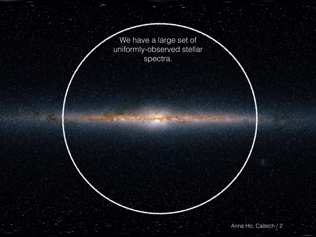
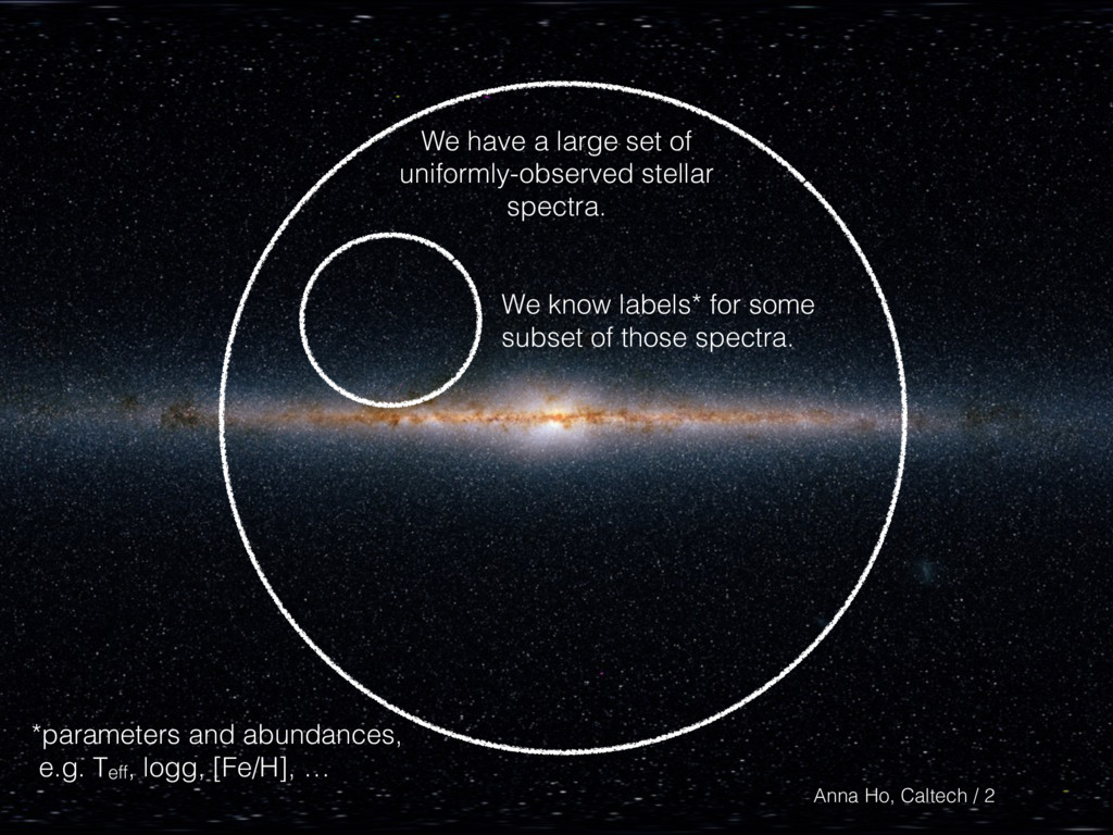
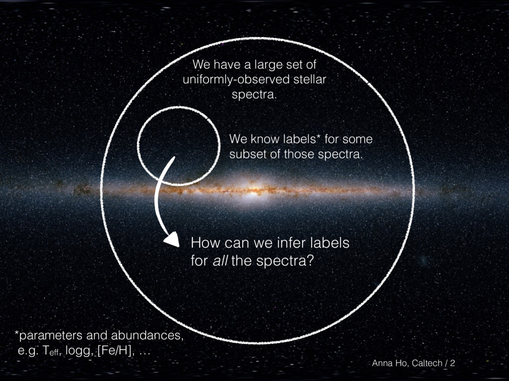
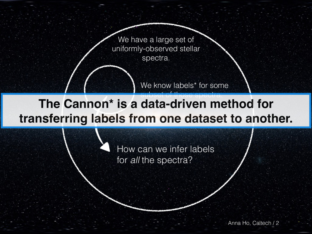
have a large set of uniformly-observed stellar spectra. We know labels* for some subset of those spectra. *parameters and abundances, e.g. Teff, logg, [Fe/H], … 2 Anna Ho, Caltech /
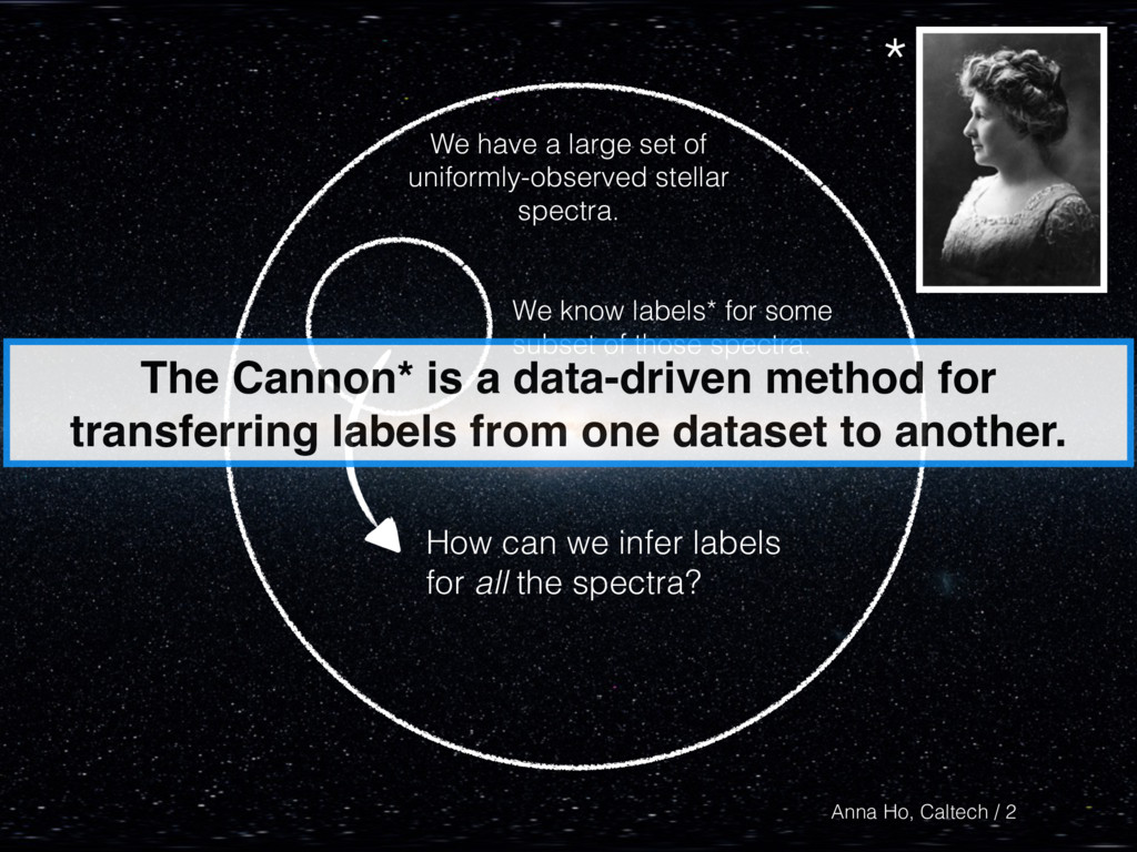
have a large set of uniformly-observed stellar spectra. We know labels* for some subset of those spectra. The Cannon* is a data-driven method for transferring labels from one dataset to another. 2 Anna Ho, Caltech /
have a large set of uniformly-observed stellar spectra. * We know labels* for some subset of those spectra. 2 Anna Ho, Caltech / The Cannon* is a data-driven method for transferring labels from one dataset to another.
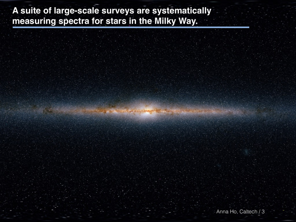
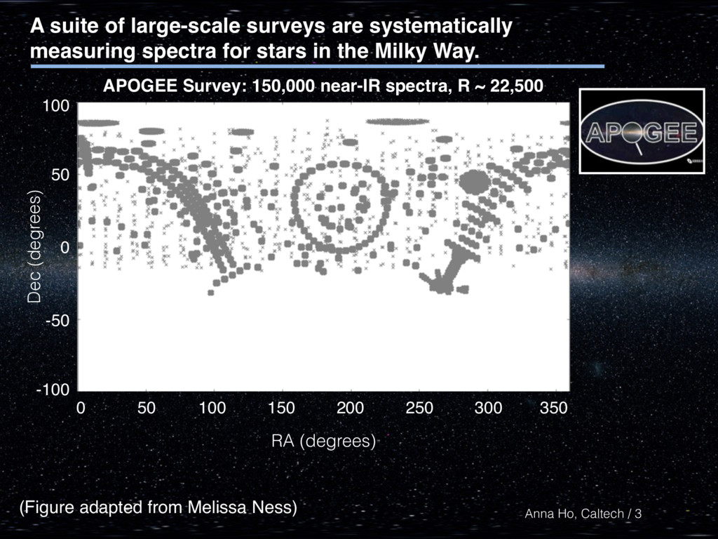
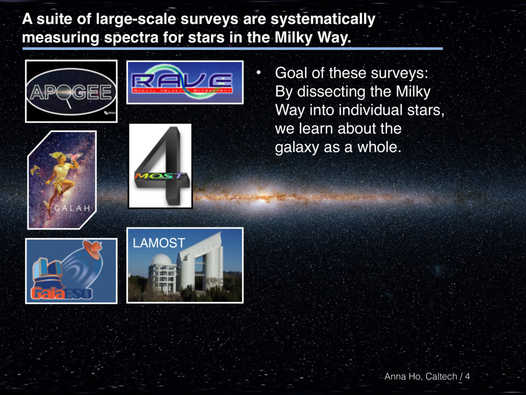
50 150 200 250 300 350 0 -100 -50 0 50 100 APOGEE Survey: 150,000 near-IR spectra, R ~ 22,500 (Figure adapted from Melissa Ness) A suite of large-scale surveys are systematically measuring spectra for stars in the Milky Way.
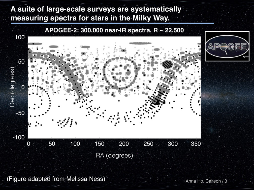
150 200 250 300 350 0 -100 -50 0 50 100 APOGEE-2: 300,000 near-IR spectra, R ~ 22,500 (Figure adapted from Melissa Ness) A suite of large-scale surveys are systematically measuring spectra for stars in the Milky Way. 3
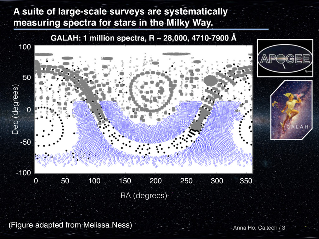
150 200 250 300 350 0 -100 -50 0 50 100 APOGEE Survey: 150,000 near-IR spectra, R ~ 22,500 GALAH: 1 million spectra, R ~ 28,000, 4710-7900 Å (Figure adapted from Melissa Ness) A suite of large-scale surveys are systematically measuring spectra for stars in the Milky Way. 3
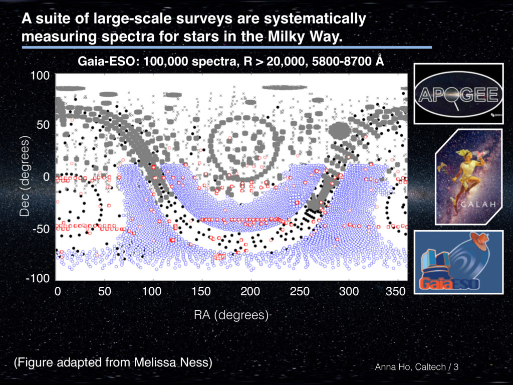
150 200 250 300 350 0 -100 -50 0 50 100 APOGEE Survey: 150,000 near-IR spectra, R ~ 22,500 Gaia-ESO: 100,000 spectra, R > 20,000, 5800-8700 Å (Figure adapted from Melissa Ness) A suite of large-scale surveys are systematically measuring spectra for stars in the Milky Way. 3
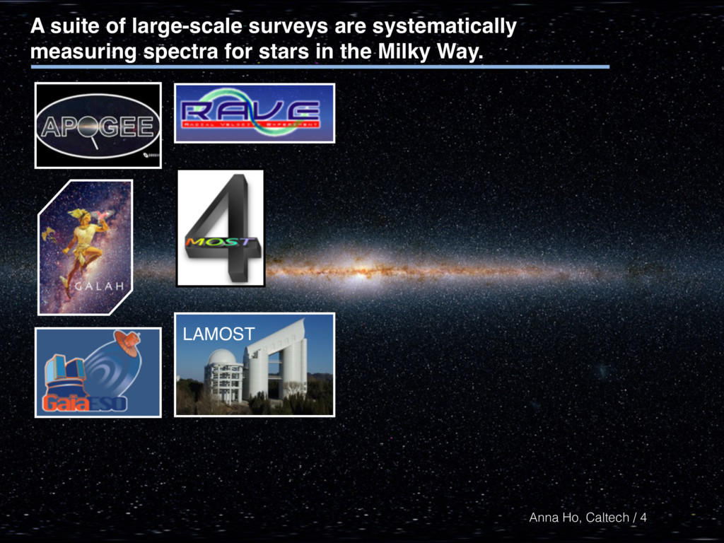
are systematically measuring spectra for stars in the Milky Way. • Goal of these surveys: By dissecting the Milky Way into individual stars, we learn about the galaxy as a whole. 4
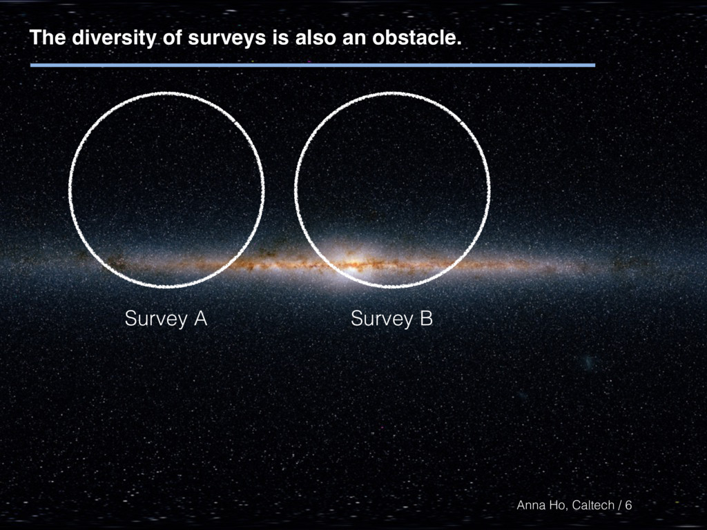
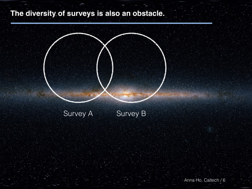
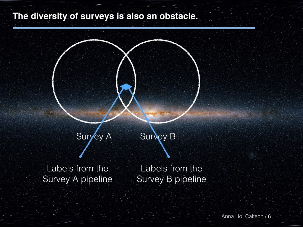
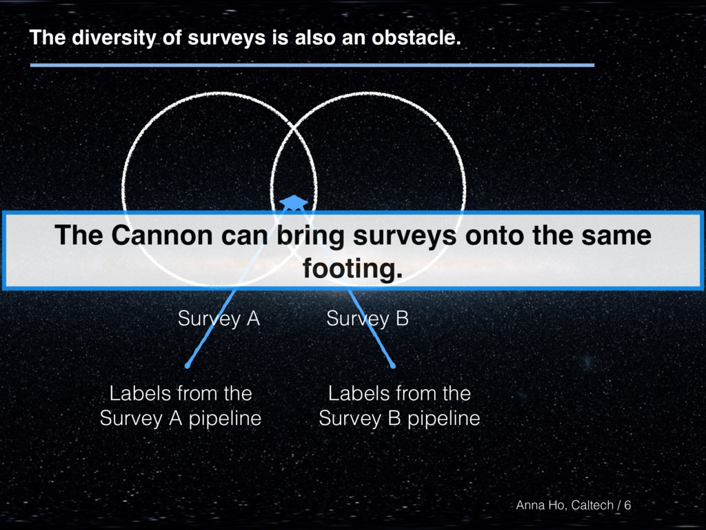
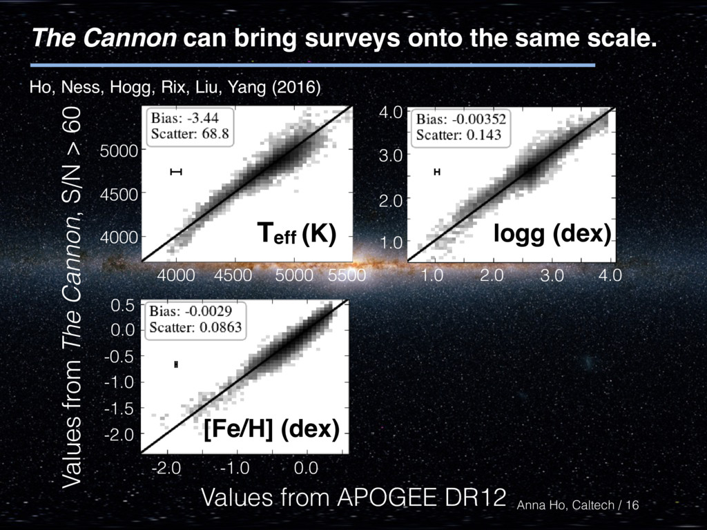
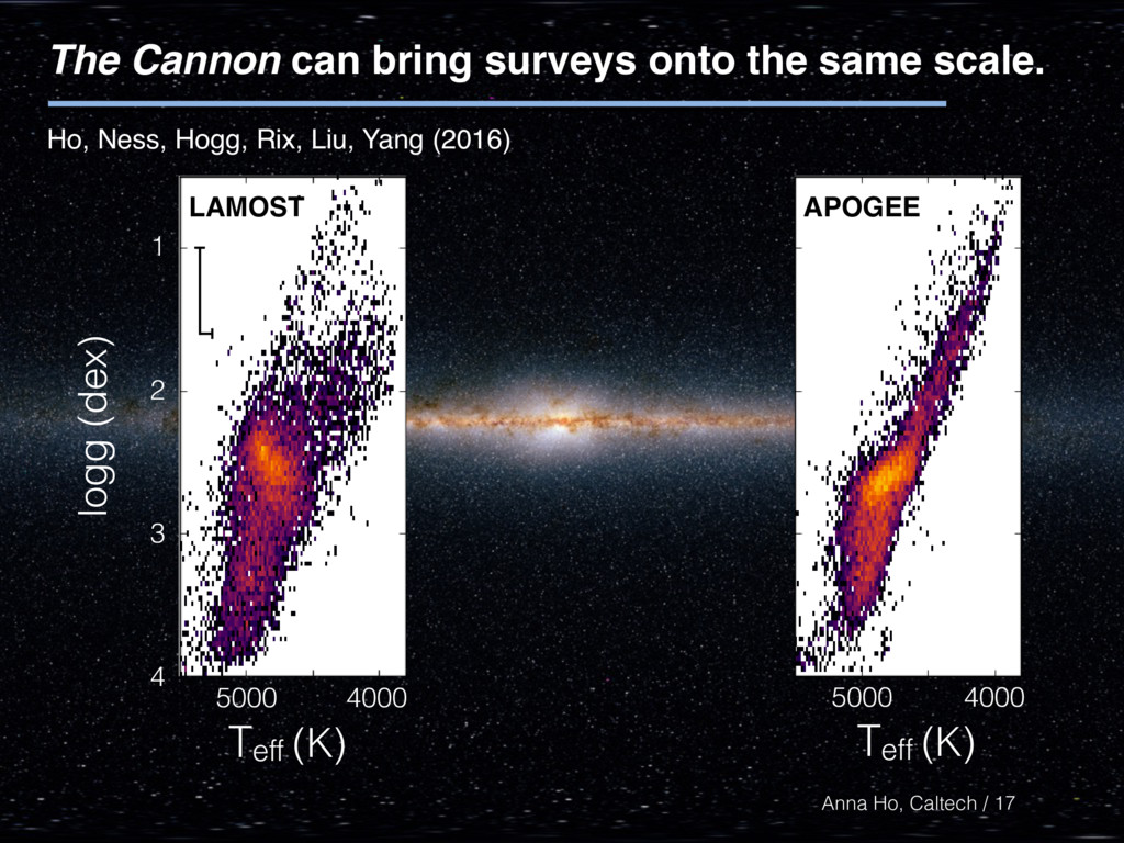
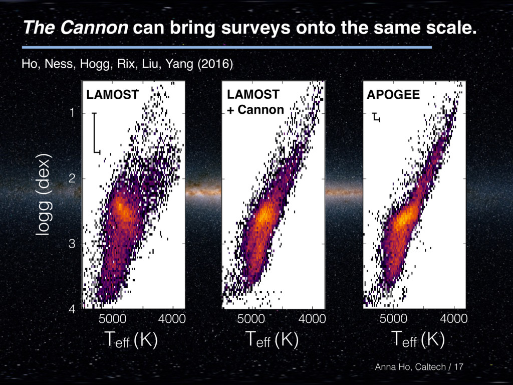
of surveys is also an obstacle. Labels from the Survey A pipeline Labels from the Survey B pipeline The Cannon can bring surveys onto the same footing. 6
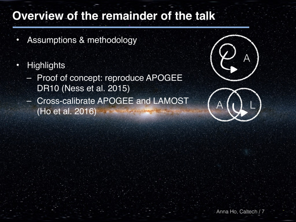
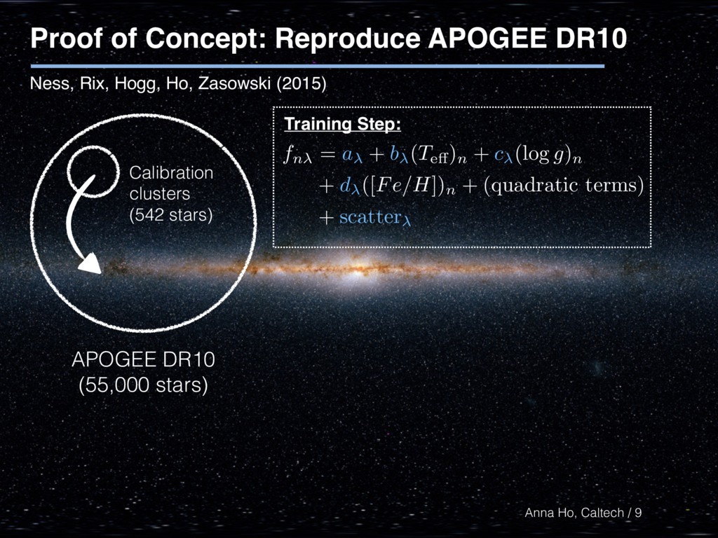
talk • Assumptions & methodology • Highlights – Proof of concept: reproduce APOGEE DR10 (Ness et al. 2015) – Cross-calibrate APOGEE and LAMOST (Ho et al. 2016) A L A 7
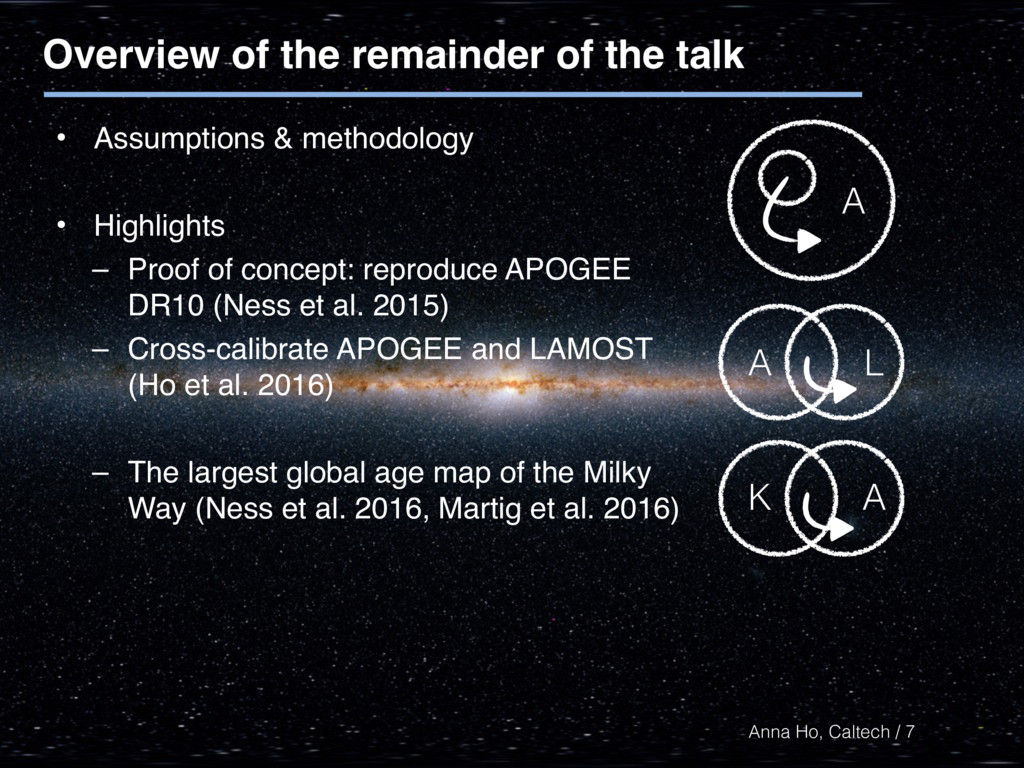
talk • Assumptions & methodology • Highlights – Proof of concept: reproduce APOGEE DR10 (Ness et al. 2015) – Cross-calibrate APOGEE and LAMOST (Ho et al. 2016) – The largest global age map of the Milky Way (Ness et al. 2016, Martig et al. 2016) A L A K A 7
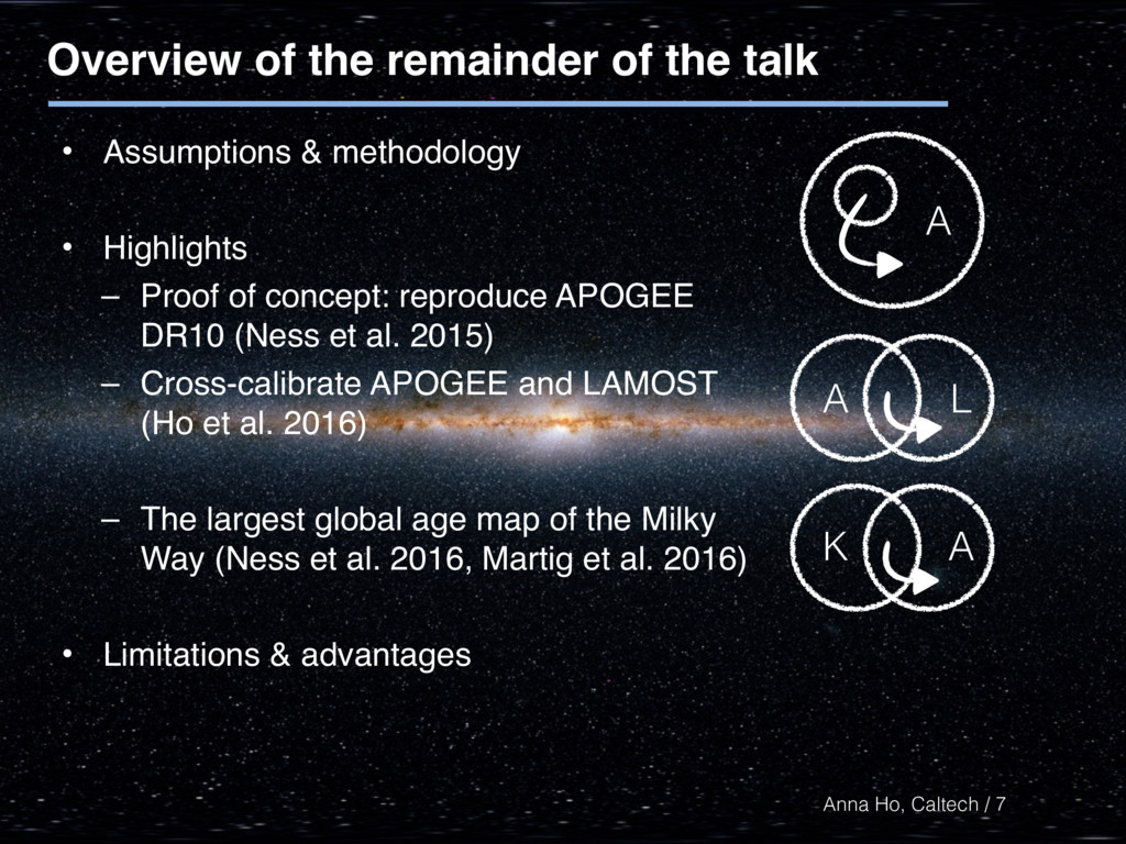
talk • Assumptions & methodology • Highlights – Proof of concept: reproduce APOGEE DR10 (Ness et al. 2015) – Cross-calibrate APOGEE and LAMOST (Ho et al. 2016) – The largest global age map of the Milky Way (Ness et al. 2016, Martig et al. 2016) • Limitations & advantages A A L K A 7
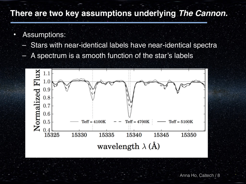
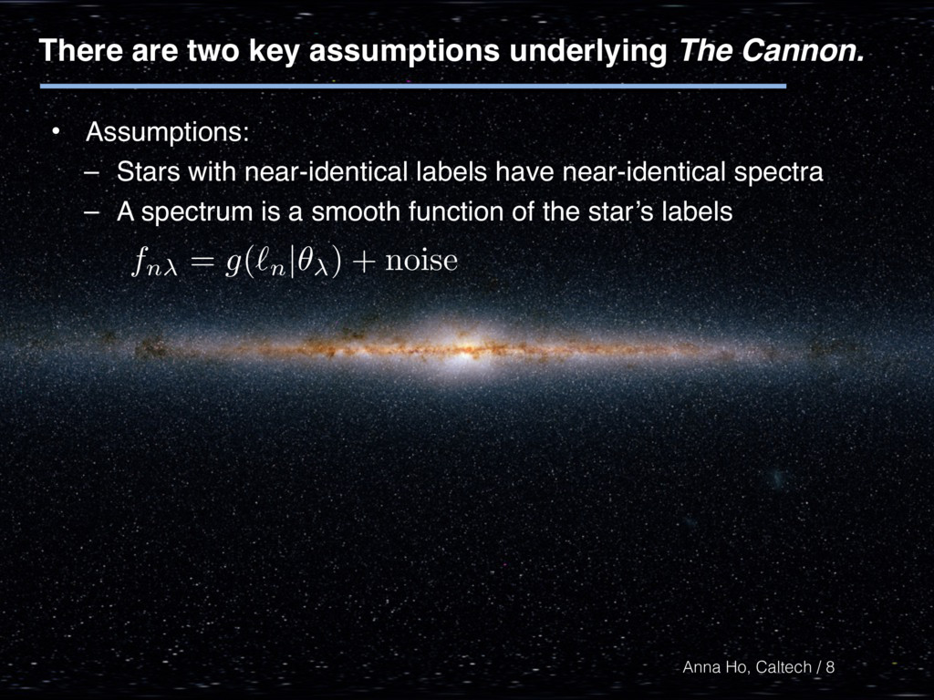
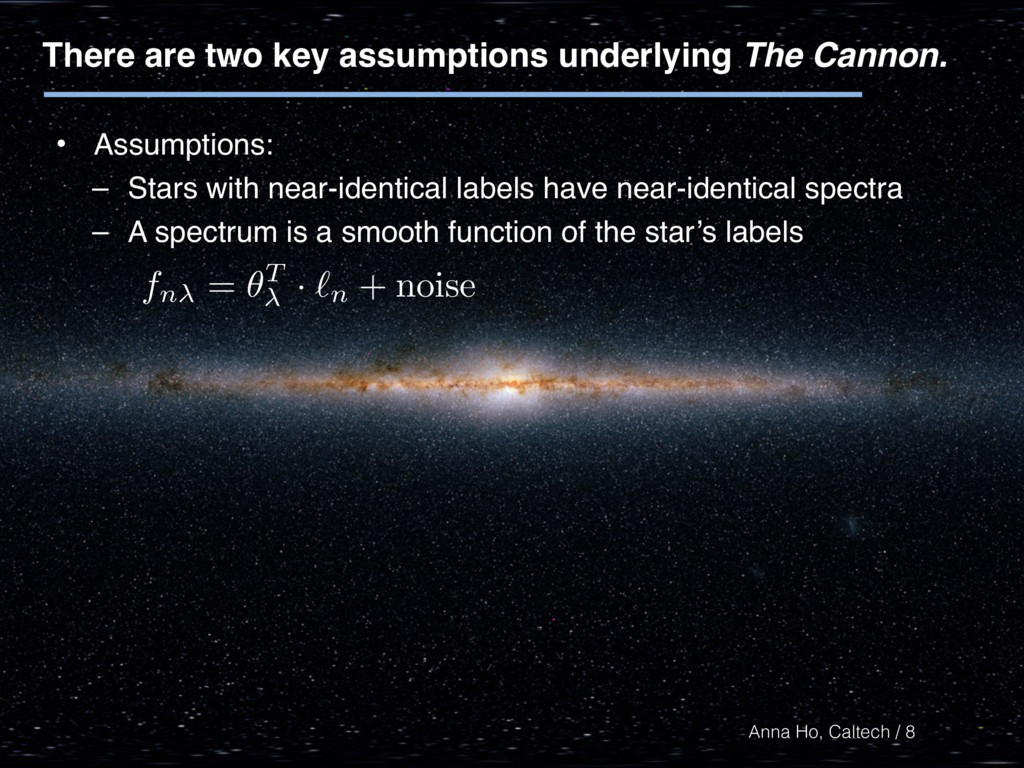
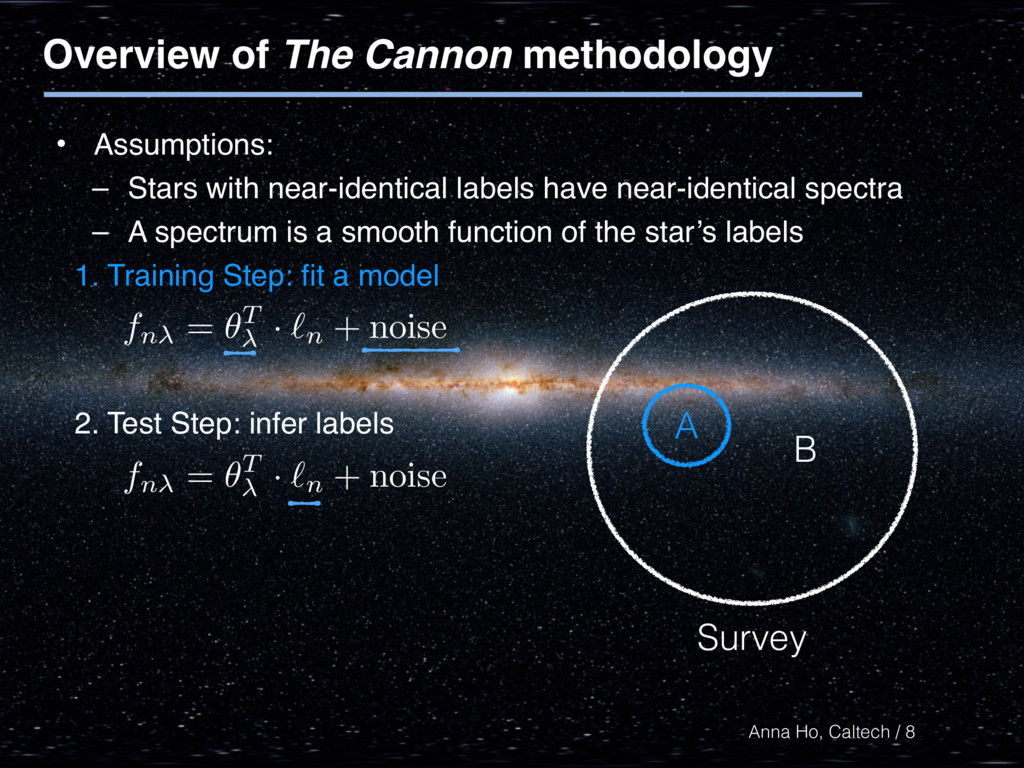
labels have near-identical spectra – A spectrum is a smooth function of the star’s labels fn = g ( `n |✓ ) + noise There are two key assumptions underlying The Cannon. 8
labels have near-identical spectra – A spectrum is a smooth function of the star’s labels There are two key assumptions underlying The Cannon. 8 fn = ✓T · `n + noise
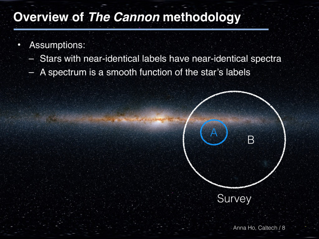
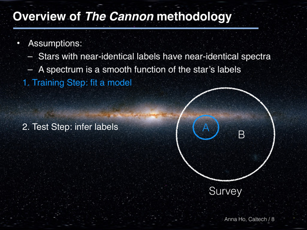
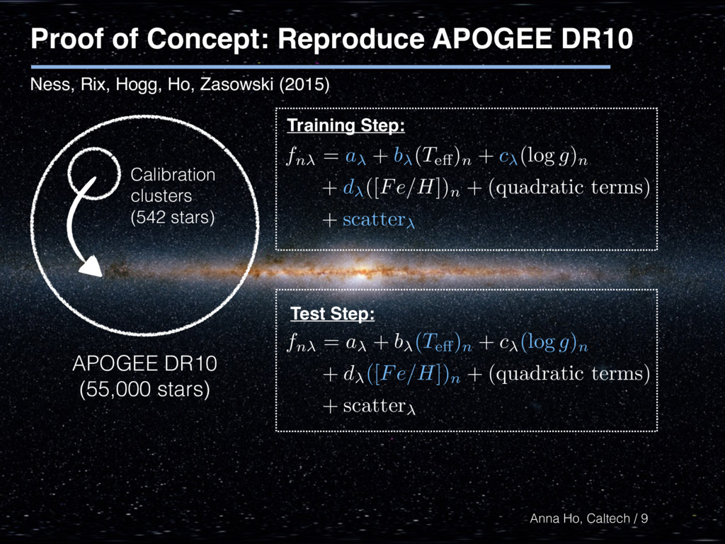
labels have near-identical spectra – A spectrum is a smooth function of the star’s labels 1. Training Step: fit a model 2. Test Step: infer labels Overview of The Cannon methodology Survey A B 8
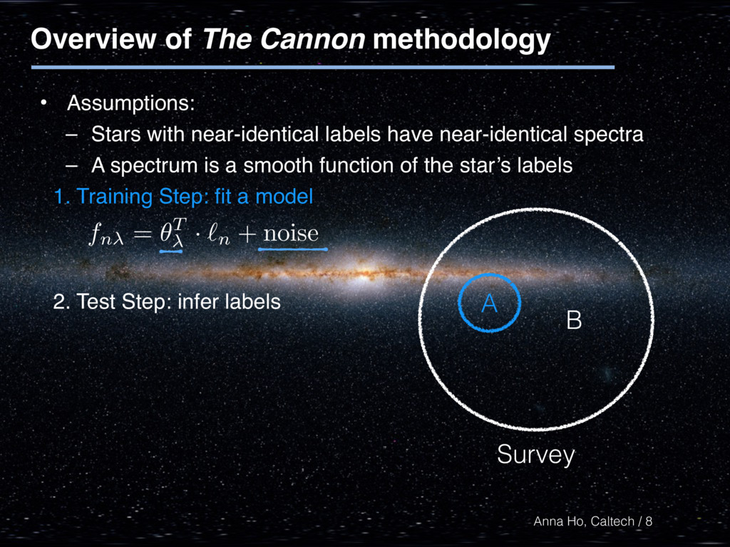
labels have near-identical spectra – A spectrum is a smooth function of the star’s labels 1. Training Step: fit a model Overview of The Cannon methodology Survey A B 2. Test Step: infer labels fn = ✓T · `n + noise 8
labels have near-identical spectra – A spectrum is a smooth function of the star’s labels 1. Training Step: fit a model 2. Test Step: infer labels Overview of The Cannon methodology Survey A B fn = ✓T · `n + noise fn = ✓T · `n + noise 8
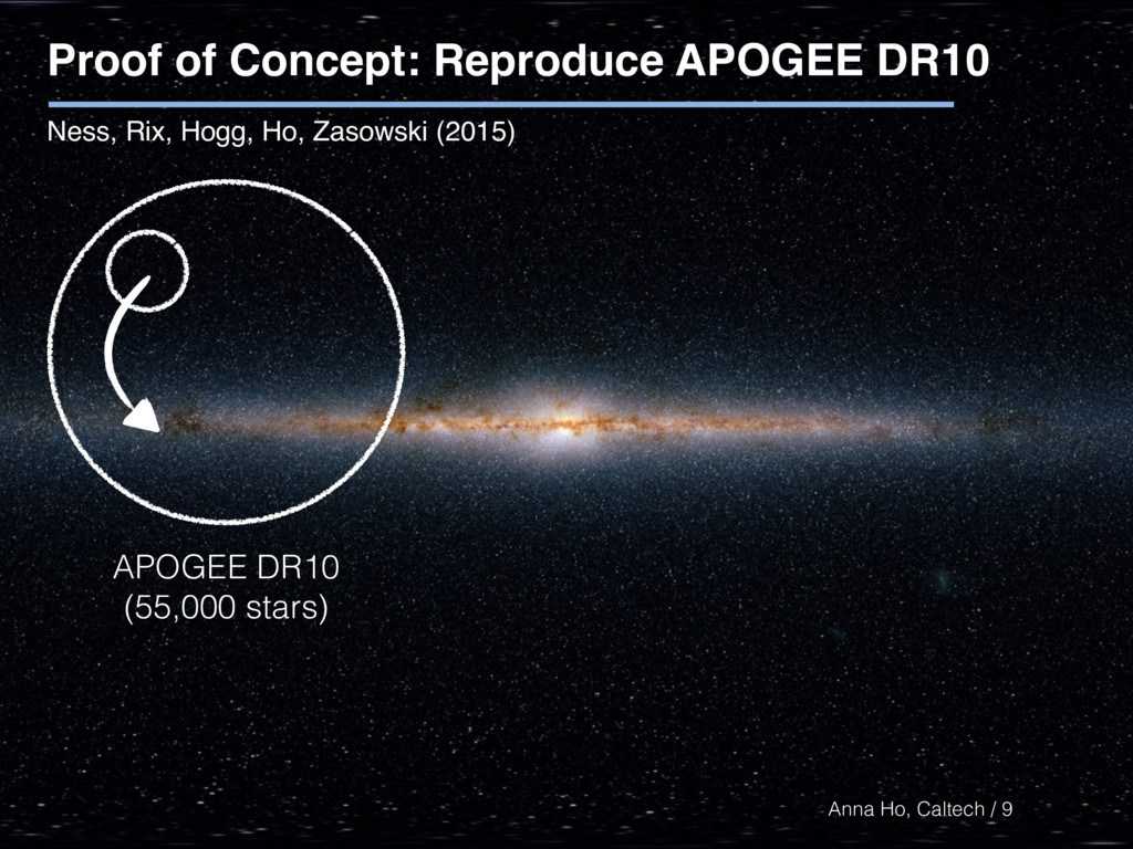
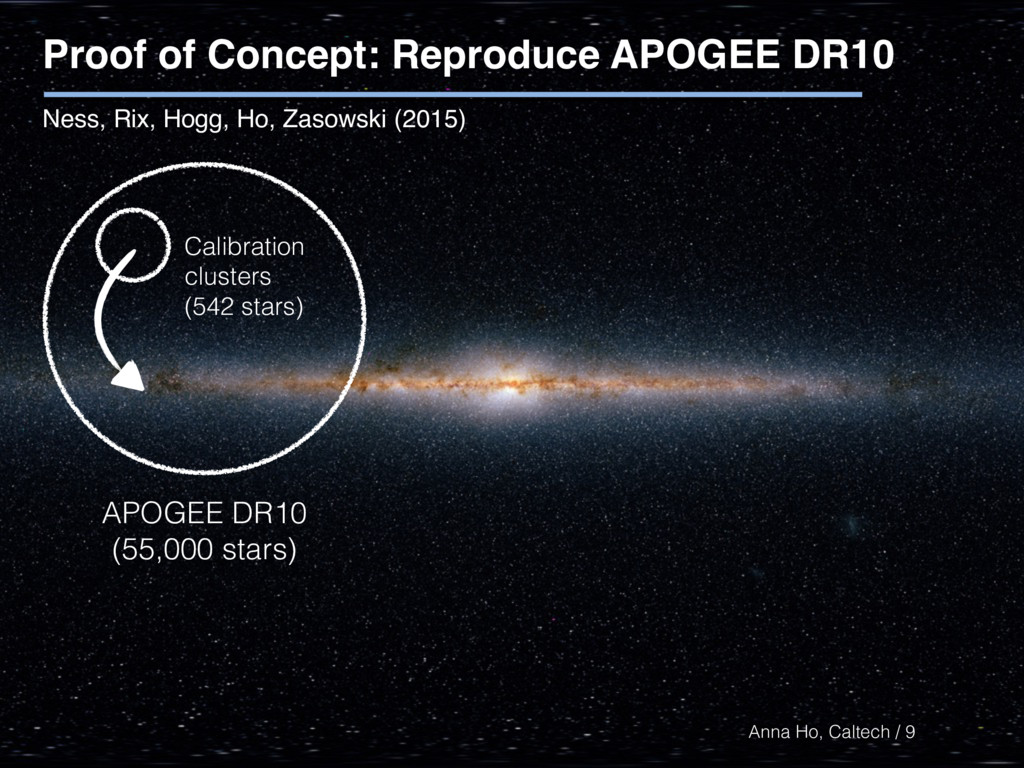
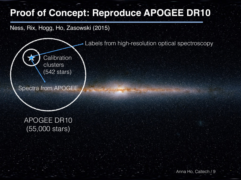
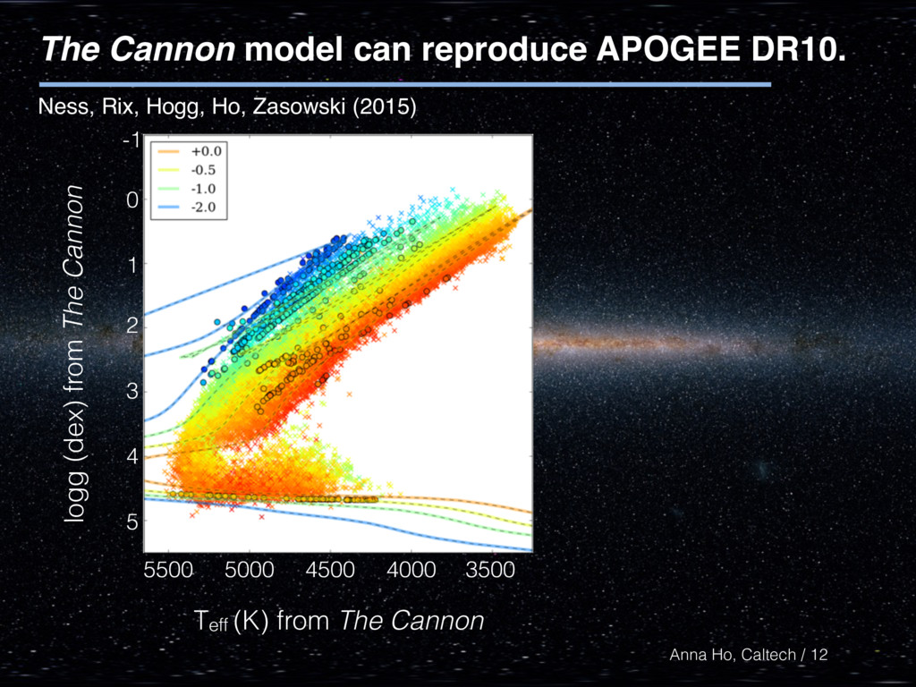
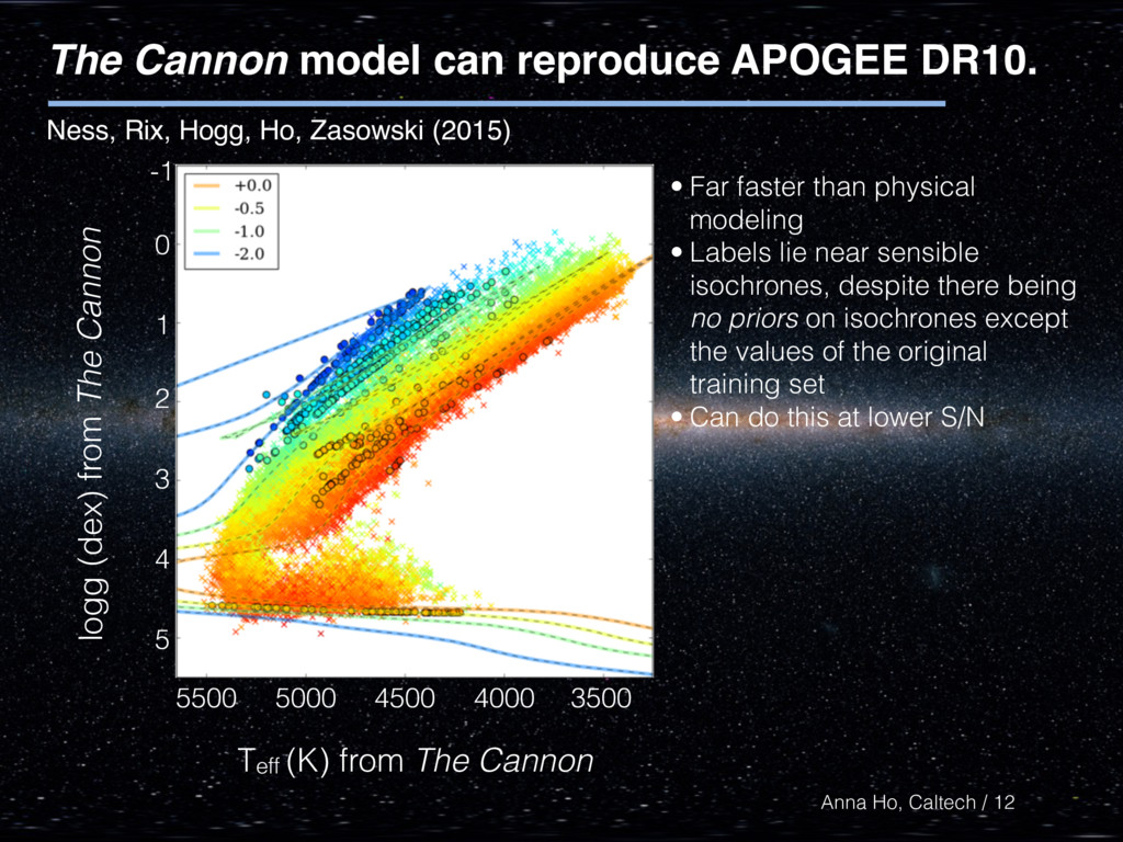
DR10. Ness, Rix, Hogg, Ho, Zasowski (2015) Teff (K) from The Cannon logg (dex) from The Cannon 4000 3500 5000 4500 5500 5 4 3 2 1 0 -1 12 • Far faster than physical modeling • Labels lie near sensible isochrones, despite there being no priors on isochrones except the values of the original training set • Can do this at lower S/N
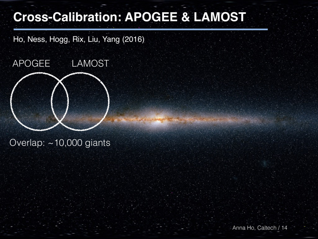
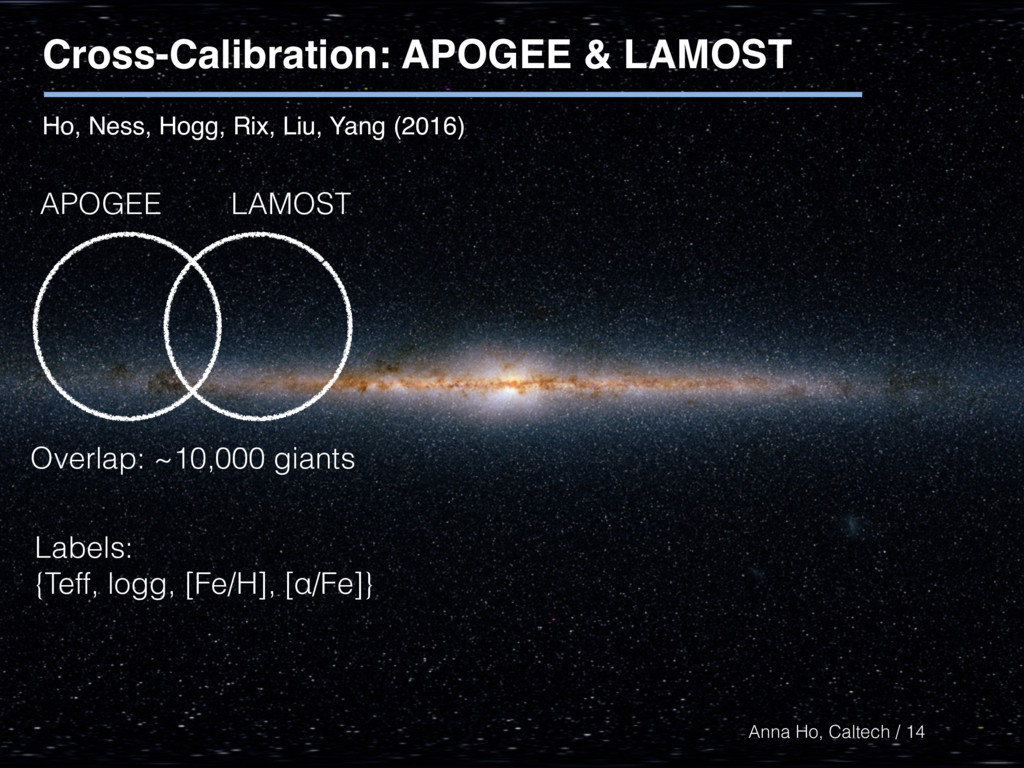
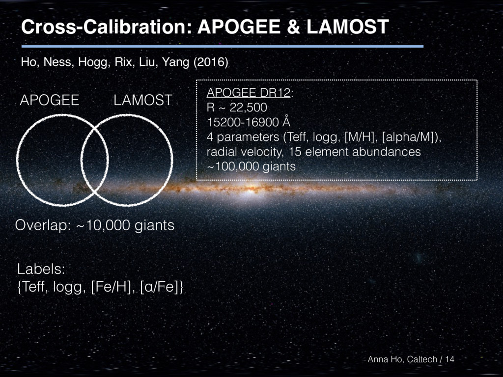
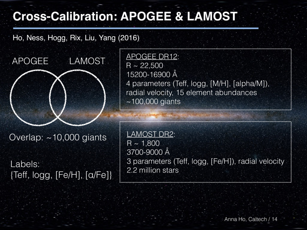
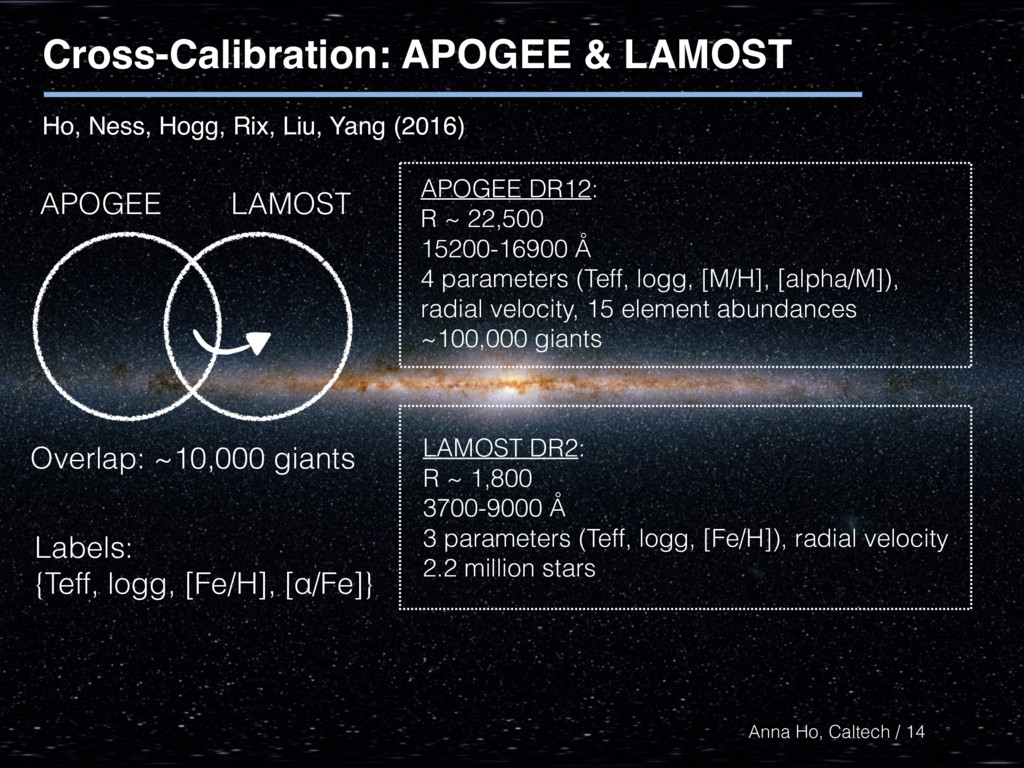
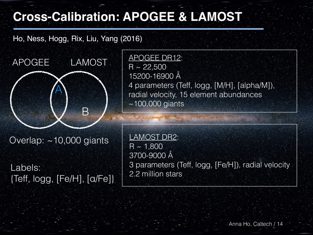
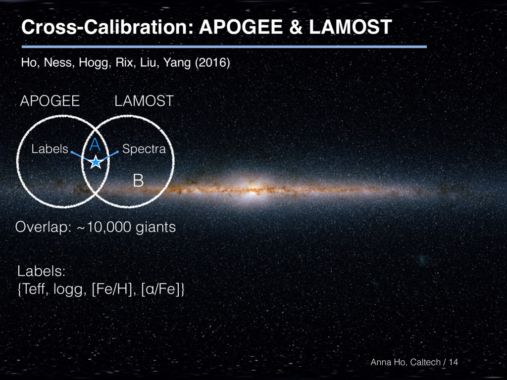
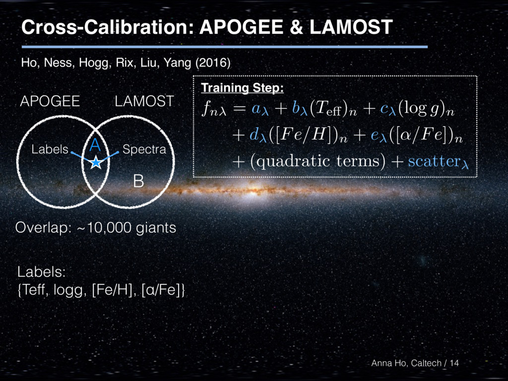
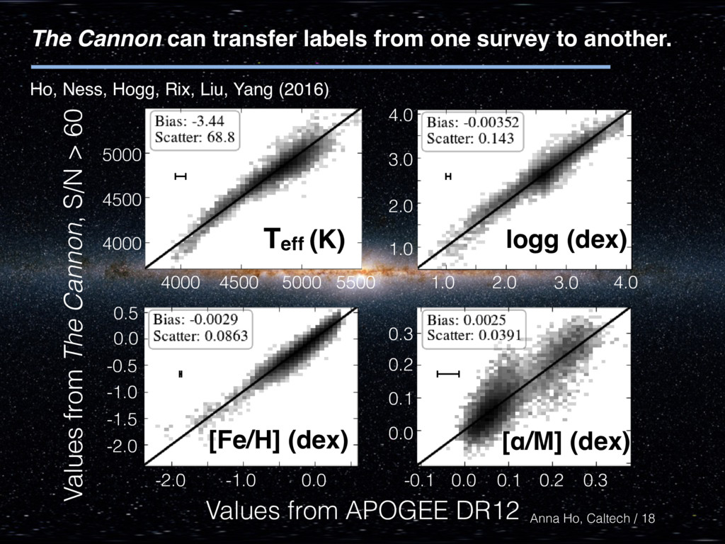
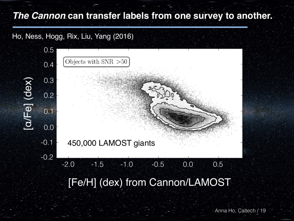
Hogg, Rix, Liu, Yang (2016) Overlap: ~10,000 giants APOGEE LAMOST Spectra Labels fn = a + b ( Te↵)n + c (log g )n + d ([ Fe/H ])n + e ([ ↵/Fe ])n + (quadratic terms) + scatter Training Step: A B Labels: {Teff, logg, [Fe/H], [α/Fe]} 14
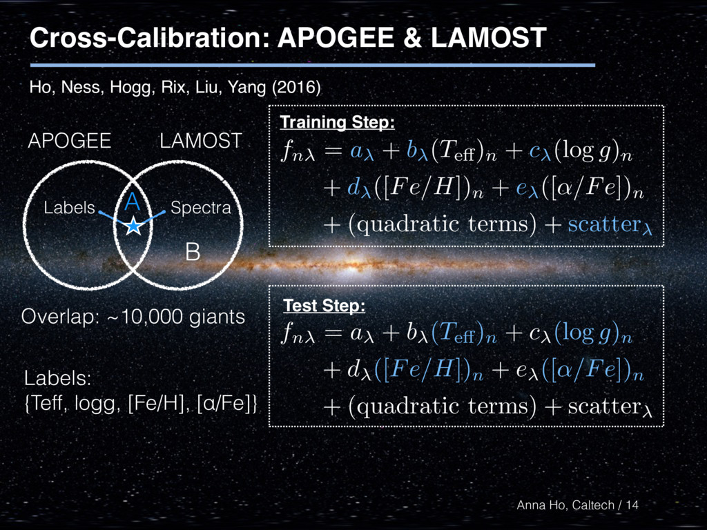
Hogg, Rix, Liu, Yang (2016) Overlap: ~10,000 giants APOGEE LAMOST Spectra Labels fn = a + b ( Te↵)n + c (log g )n + d ([ Fe/H ])n + e ([ ↵/Fe ])n + (quadratic terms) + scatter fn = a + b ( Te↵)n + c (log g )n + d ([ Fe/H ])n + e ([ ↵/Fe ])n + (quadratic terms) + scatter Training Step: Test Step: A B Labels: {Teff, logg, [Fe/H], [α/Fe]} 14
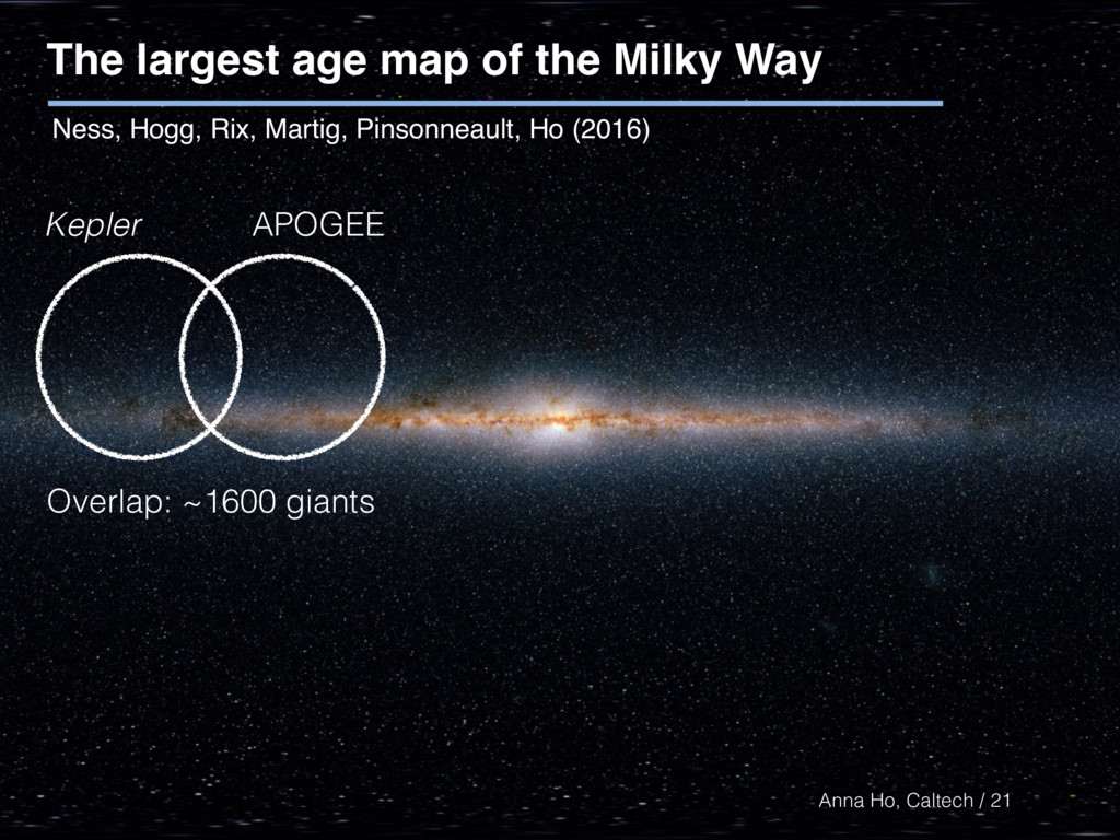
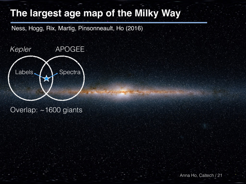
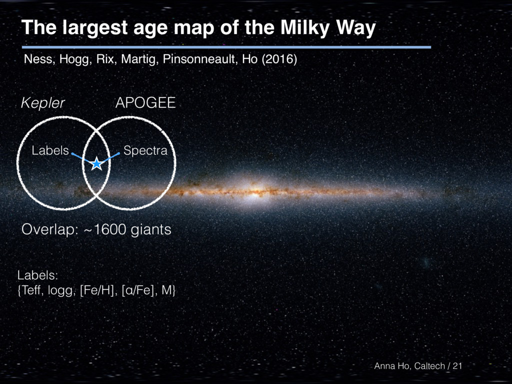
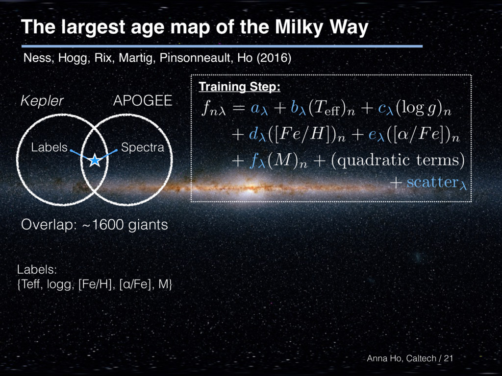
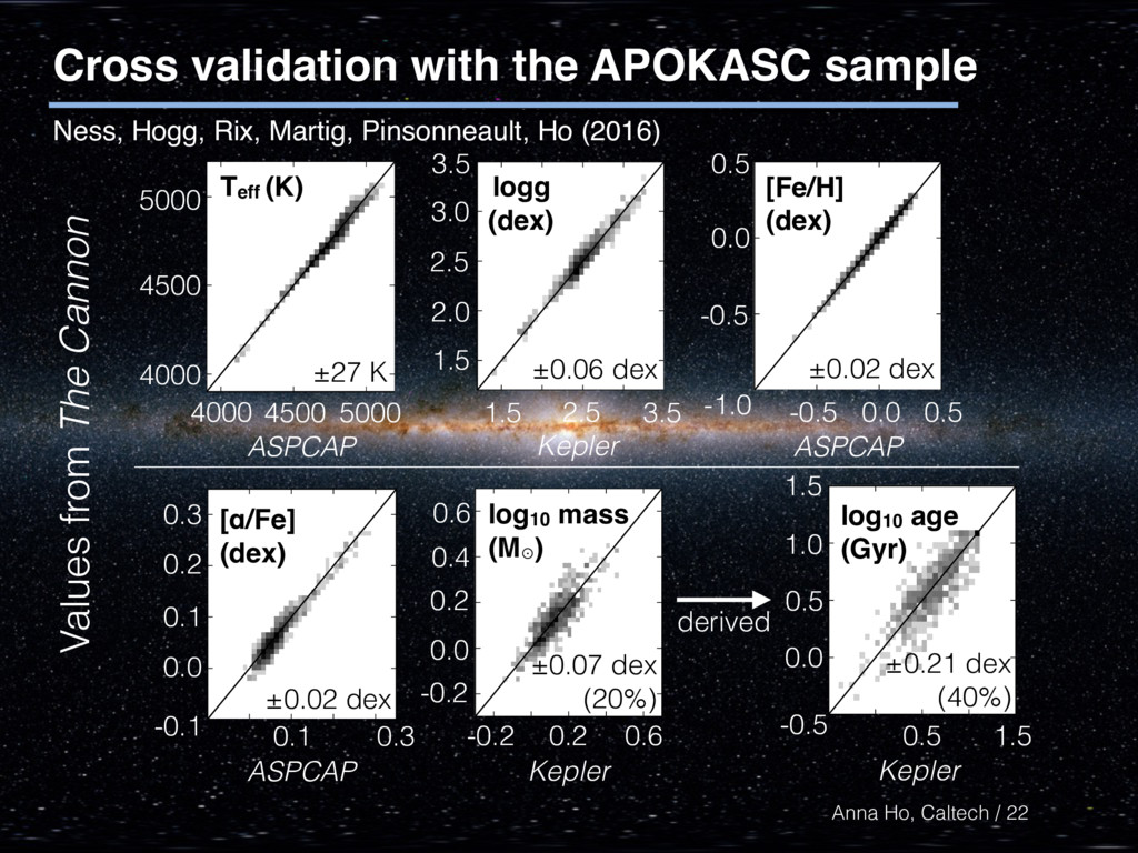
Milky Way Overlap: ~1600 giants Kepler APOGEE Spectra Labels fn = a + b ( Te↵)n + c (log g )n + d ([ Fe/H ])n + e ([ ↵/Fe ])n + f ( M )n + (quadratic terms) + sca fn = a + b ( Te↵)n + c (log g )n + d ([ Fe/H ])n + e ([ ↵/Fe ])n + f ( M )n + (quadratic terms) + scatter Training Step: Labels: {Teff, logg, [Fe/H], [α/Fe], M} 21 Ness, Hogg, Rix, Martig, Pinsonneault, Ho (2016)
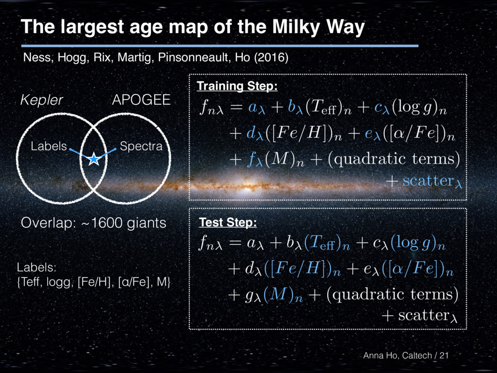
Milky Way Overlap: ~1600 giants Kepler APOGEE Spectra Labels fn = a + b ( Te↵)n + c (log g )n + d ([ Fe/H ])n + e ([ ↵/Fe ])n + f ( M )n + (quadratic terms) + sca fn = a + b ( Te↵)n + c (log g )n + d ([ Fe/H ])n + e ([ ↵/Fe ])n + f ( M )n + (quadratic terms) + scatter Training Step: Test Step: fn = a + b ( Te↵)n + c (log g )n + d ([ Fe/H ])n + e ([ ↵/Fe ])n + g ( M )n + (quadratic terms) + sca fn = a + b ( Te↵)n + c (log g )n + d ([ Fe/H ])n + e ([ ↵/Fe ])n + g ( M )n + (quadratic terms) + scatter 21 Labels: {Teff, logg, [Fe/H], [α/Fe], M} Ness, Hogg, Rix, Martig, Pinsonneault, Ho (2016)
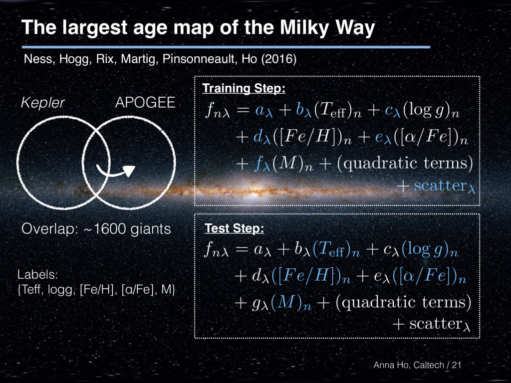
Milky Way Overlap: ~1600 giants Kepler APOGEE fn = a + b ( Te↵)n + c (log g )n + d ([ Fe/H ])n + e ([ ↵/Fe ])n + f ( M )n + (quadratic terms) + sca fn = a + b ( Te↵)n + c (log g )n + d ([ Fe/H ])n + e ([ ↵/Fe ])n + f ( M )n + (quadratic terms) + scatter Training Step: Test Step: fn = a + b ( Te↵)n + c (log g )n + d ([ Fe/H ])n + e ([ ↵/Fe ])n + g ( M )n + (quadratic terms) + sca fn = a + b ( Te↵)n + c (log g )n + d ([ Fe/H ])n + e ([ ↵/Fe ])n + g ( M )n + (quadratic terms) + scatter 21 Labels: {Teff, logg, [Fe/H], [α/Fe], M} Ness, Hogg, Rix, Martig, Pinsonneault, Ho (2016)
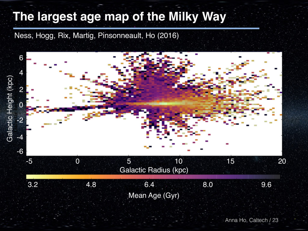
Galactic Height (kpc) -5 0 5 10 15 20 -6 -4 -2 0 2 4 6 Mean Age (Gyr) 9.6 3.2 6.4 4.8 8.0 The largest age map of the Milky Way Anna Ho, Caltech / 23 Ness, Hogg, Rix, Martig, Pinsonneault, Ho (2016)
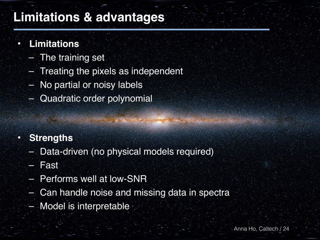
The training set – Treating the pixels as independent – No partial or noisy labels – Quadratic order polynomial 24 • Strengths – Data-driven (no physical models required) – Fast – Performs well at low-SNR – Can handle noise and missing data in spectra – Model is interpretable
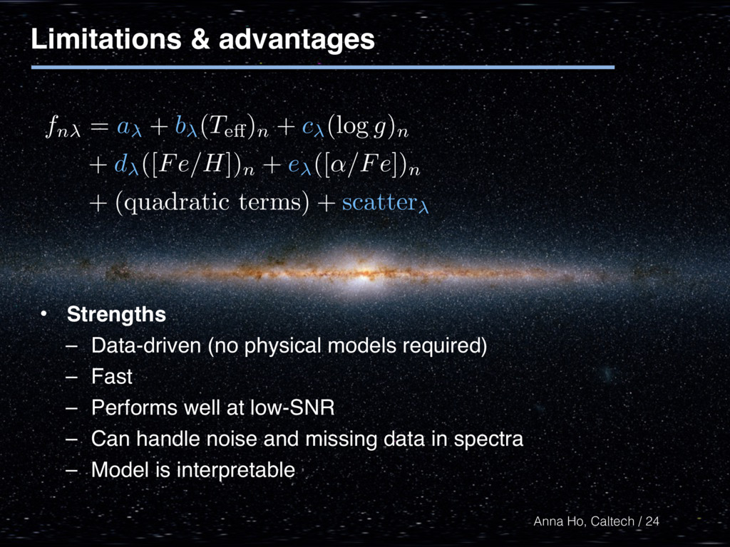
+ b ( Te↵)n + c (log g )n + d ([ Fe/H ])n + e ([ ↵/Fe ])n + (quadratic terms) + scatter 24 • Strengths – Data-driven (no physical models required) – Fast – Performs well at low-SNR – Can handle noise and missing data in spectra – Model is interpretable
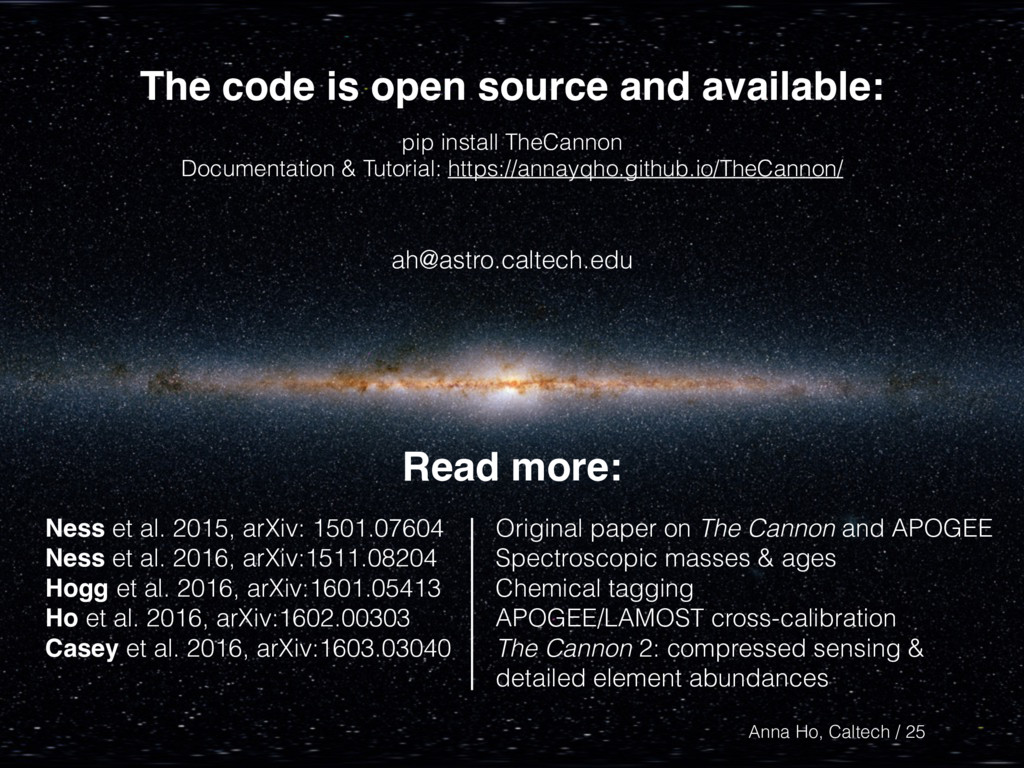
Documentation & Tutorial: https://annayqho.github.io/TheCannon/ 25 Anna Ho, Caltech / Read more: Ness et al. 2015, arXiv: 1501.07604 Ness et al. 2016, arXiv:1511.08204 Hogg et al. 2016, arXiv:1601.05413 Ho et al. 2016, arXiv:1602.00303 Casey et al. 2016, arXiv:1603.03040 Original paper on The Cannon and APOGEE Spectroscopic masses & ages Chemical tagging APOGEE/LAMOST cross-calibration The Cannon 2: compressed sensing & detailed element abundances [email protected]
![Anna Ho, Caltech / “Labels”: {M, L, Teff, logg, [Fe/H],](https://files.speakerdeck.com/presentations/e9c9d1451cc942e495aa728cbd6ab36e/slide_19.jpg)
![APOGEE [α/M] 100,000 giants](https://files.speakerdeck.com/presentations/e9c9d1451cc942e495aa728cbd6ab36e/slide_62.jpg)
![APOGEE [α/M] LAMOST [α/M] 100,000 giants + 450,000 giants](https://files.speakerdeck.com/presentations/e9c9d1451cc942e495aa728cbd6ab36e/slide_63.jpg)