Implementing Hamiltonian Monte Carlo for Efficient Bayesian Evolutionary Analysis

Talk at Allan Wilson Centre Annual Meeting 2015

Transcript

1. Introduction Methods Results Conclusion Implementing Hamiltonian Monte Carlo for Efficient Bayesian Evolutionary Analysis Arman Bilge abil933@aucklanduni.ac.nz Computational Evolution Group The University of Auckland 21 October 2015
2. Introduction Methods Results Conclusion Motivation Bayesian statistics has transformed evolutionary biology Divergence dating and clock rate estimation Inference of demographics and population history parameters Phylodynamic and epidemiological parameters
3. Introduction Methods Results Conclusion Motivation Bayesian statistics has transformed evolutionary biology Divergence dating and clock rate estimation Inference of demographics and population history parameters Phylodynamic and epidemiological parameters Want to sample phylogenetic tree and model parameters according to their probability given the data P (T , θ | D)
4. Introduction Methods Results Conclusion Motivation Bayesian statistics has transformed evolutionary biology Divergence dating and clock rate estimation Inference of demographics and population history parameters Phylodynamic and epidemiological parameters Want to sample phylogenetic tree and model parameters according to their probability given the data P (T , θ | D) Need a way to efficiently explore different models
5. Introduction Methods Results Conclusion Current State-of-the-Art Metropolis–Hastings Markov chain Monte Carlo (MCMC) Imagine a robot taking a random walk
6. Introduction Methods Results Conclusion Current State-of-the-Art Metropolis–Hastings Markov chain Monte Carlo (MCMC) Imagine a robot taking a random walk That’s just unbearably slow
7. Introduction Methods Results Conclusion Current State-of-the-Art Metropolis–Hastings Markov chain Monte Carlo (MCMC) Imagine a robot taking a random walk That’s just unbearably slow But suppose we gave our robot a pair of skis...
8. Introduction Methods Results Conclusion Cooker, an Aspiring Skier
9. Introduction Methods Results Conclusion Physics Primer (Hamiltonian Dynamics) Definition Let q be the robot’s position v be its velocity M be its mass U (q) be its potential energy K (p) be its kinetic energy Then the Hamiltonian H is H (q, p) = U (q) + K (p) U (q) q p = Mv K (p) = 1 2 pT M−1p
10. Introduction Methods Results Conclusion Physics Primer (Hamiltonian Dynamics) Definition Let q be the robot’s position v be its velocity M be its mass U (q) be its potential energy K (p) be its kinetic energy Then the Hamiltonian H is H (q, p) = U (q) + K (p) H is conserved Simulates robot’s motion U (q) q p = Mv K (p) = 1 2 pT M−1p
11. Introduction Methods Results Conclusion Hamiltonian Moves Flip direction
12. Introduction Methods Results Conclusion Hamiltonian Moves Ski!
13. Introduction Methods Results Conclusion Hamiltonian Moves Push in a random direction
14. Introduction Methods Results Conclusion Hamiltonian Monte Carlo How do we make a stats problem into a physics problem?
15. Introduction Methods Results Conclusion Hamiltonian Monte Carlo How do we make a stats problem into a physics problem? Every location q maps to some model parameters
16. Introduction Methods Results Conclusion Hamiltonian Monte Carlo How do we make a stats problem into a physics problem? Every location q maps to some model parameters Elevation at q is − log P (T , θ | D)
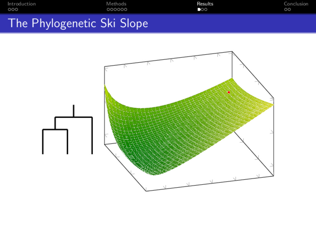
17. Introduction Methods Results Conclusion Hamiltonian Monte Carlo How do we make a stats problem into a physics problem? Every location q maps to some model parameters Elevation at q is − log P (T , θ | D) Locations with high elevation have low probability Locations with low elevation have high probability
18. Introduction Methods Results Conclusion Hamiltonian Monte Carlo How do we make a stats problem into a physics problem? Every location q maps to some model parameters Elevation at q is − log P (T , θ | D) Locations with high elevation have low probability Locations with low elevation have high probability Done!
19. Introduction Methods Results Conclusion Hamiltonian Monte Carlo Running a physics simulator seems like a lot of work! Why should we bother?
20. Introduction Methods Results Conclusion Hamiltonian Monte Carlo Running a physics simulator seems like a lot of work! Why should we bother? Theorem (Creutz 1988) Consider a model with n variables. Then (under simplifying assumptions) the computation time is O n2 for MCMC; and O n5 4 for HMC.
21. Introduction Methods Results Conclusion Hamiltonian Monte Carlo Running a physics simulator seems like a lot of work! Why should we bother? Theorem (Creutz 1988) Consider a model with n variables. Then (under simplifying assumptions) the computation time is O n2 for MCMC; and O n5 4 for HMC. In practice this means doubling the model complexity increases computation time by 4x for MCMC <2.5x for HMC!
22. Introduction Methods Results Conclusion The Phylogenetic Ski Slope
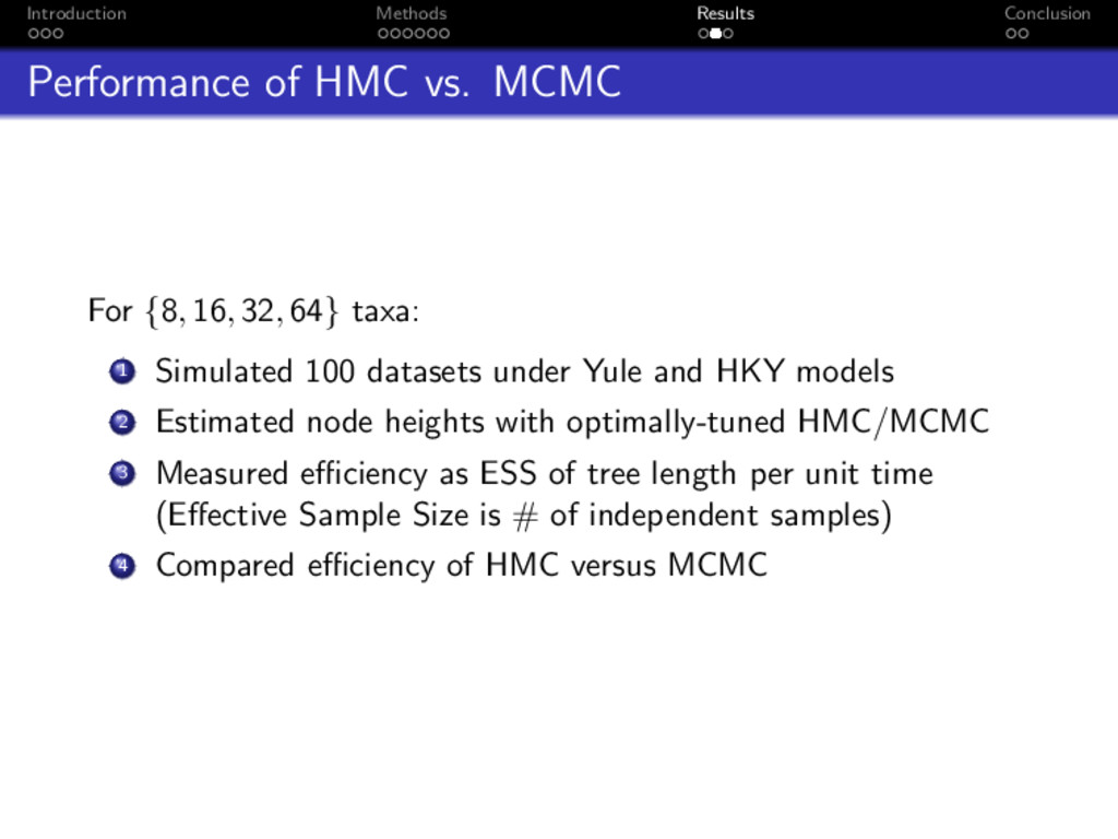
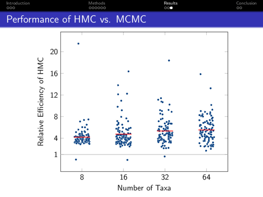
23. Introduction Methods Results Conclusion Performance of HMC vs. MCMC For {8, 16, 32, 64} taxa: 1 Simulated 100 datasets under Yule and HKY models 2 Estimated node heights with optimally-tuned HMC/MCMC 3 Measured efficiency as ESS of tree length per unit time (Effective Sample Size is # of independent samples) 4 Compared efficiency of HMC versus MCMC
24. Introduction Methods Results Conclusion Performance of HMC vs. MCMC 8 16 32 64 1 4 8 12 16 20 Number of Taxa Relative Efficiency of HMC
25. Introduction Methods Results Conclusion Concluding Remarks Conclusions HMC consistently out-performed MCMC On average, HMC was 5x more efficient than MCMC Open source implementation at http://github.com/armanbilge/B3/tree/hamilton
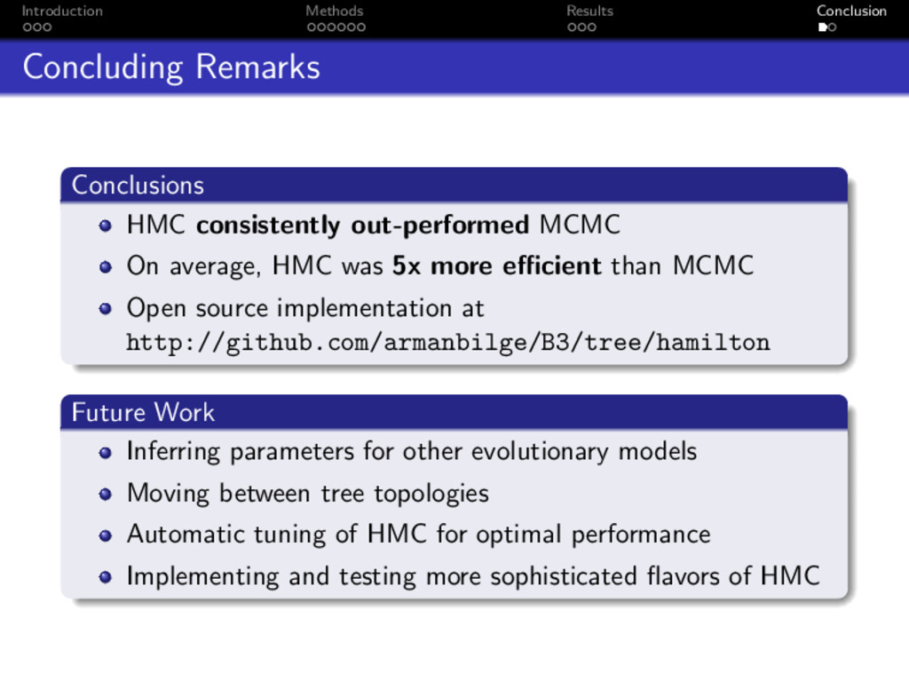
26. Introduction Methods Results Conclusion Concluding Remarks Conclusions HMC consistently out-performed MCMC On average, HMC was 5x more efficient than MCMC Open source implementation at http://github.com/armanbilge/B3/tree/hamilton Future Work Inferring parameters for other evolutionary models Moving between tree topologies Automatic tuning of HMC for optimal performance Implementing and testing more sophisticated flavors of HMC
27. Introduction Methods Results Conclusion Acknowledgements Thanks to Tim Vaughan and Alexei Drummond Members of the Computational Evolution Group Allan Wilson Centre Summer Scholarship New Zealand eScience Infrastructure References M Creutz. Physical Review D 38.4 (1988). doi:10.1103/PhysRevD.38.1228 RM Neal. Handbook of Markov Chain Monte Carlo (2011).