poliastro @ OSCW'17

Transcript

1. poliastro: an Astrodynamics library written in Python poliastro: an Astrodynamics library written in Python poli Astrodynamics in Python astro Juan Luis Cano - 2017-11-23 OSCW @ ESOC Juan Luis Cano - 2017-11-23 OSCW @ ESOC
2. 1. Introduction (2 minutes) 1. Introduction (2 minutes) What is poliastro? What is poliastro? Pure Python library for Astrodynamics Orbital element conversion, analytical and numerical propagation, interface to NEOs databases, orbital maneuvers Physical unit handling, astronomical time scales Cool documentation Version 0.8.0 released few days ago! MIT License (permissive, i.e. commercial-friendly) http://docs.poliastro.space/ (http://docs.poliastro.space/) http://docs.poliastro.space/en/v0.8.0 /changelog.html#poliastro-0-8-0-2017-11-18 (http://docs.poliastro.space /en/v0.8.0/changelog.html#poliastro-0-8-0-2017-11-18)
3. Brief history Brief history 2013: First version: Octave + FORTRAN + Python 2014: Refactor of the API, much friendlier 2015: Replace FORTRAN algorithms by Python + numba 2016: Izzo algorithm (Lambert's problem), presentation at 6th ICATT 2017: SOCIS (ESA) grant, OpenAstronomy & Astropy membership
4. Why another... How does it compare to...? How does it compare to...? Orekit: not restricted to Earth orbits, more general NASA SPICE: more lightweight, focused on interactive use, not backed by NASA
5. 2. Main features (7½ minutes) 2. Main features (7½ minutes) 2.1. First contact 2.1. First contact Interactive usage on Jupyter notebook Physical units, astronomical time scales and reference frame handling (thanks to Astropy) Orbital elements conversion (cartesian, keplerian, equinoctial) 2D and 3D visualization
6. In [2]: from poliastro.bodies import Earth from poliastro.twobody import Orbit In [3]: r = [-6045, -3490, 2500] * u.km v = [-3.457, 6.618, 2.533] * u.km / u.s ss = Orbit.from_vectors(Earth, r, v, Time.now()) ss Out[3]: 7283 x 10293 km x 153.2 deg orbit around Earth (♁) In [4]: ss.epoch Out[4]: <Time object: scale='utc' format='datetime' value=2017-11-21 23:21:46.509700> In [5]: ss.raan.to(u.deg) Out[5]: 255.27929 ∘
7. In [6]: from poliastro.plotting import plot, plot3d plot(ss, label="Sample orbit");
8. In [9]: plot3d(ss, label="Sample orbit"); Out[9]:
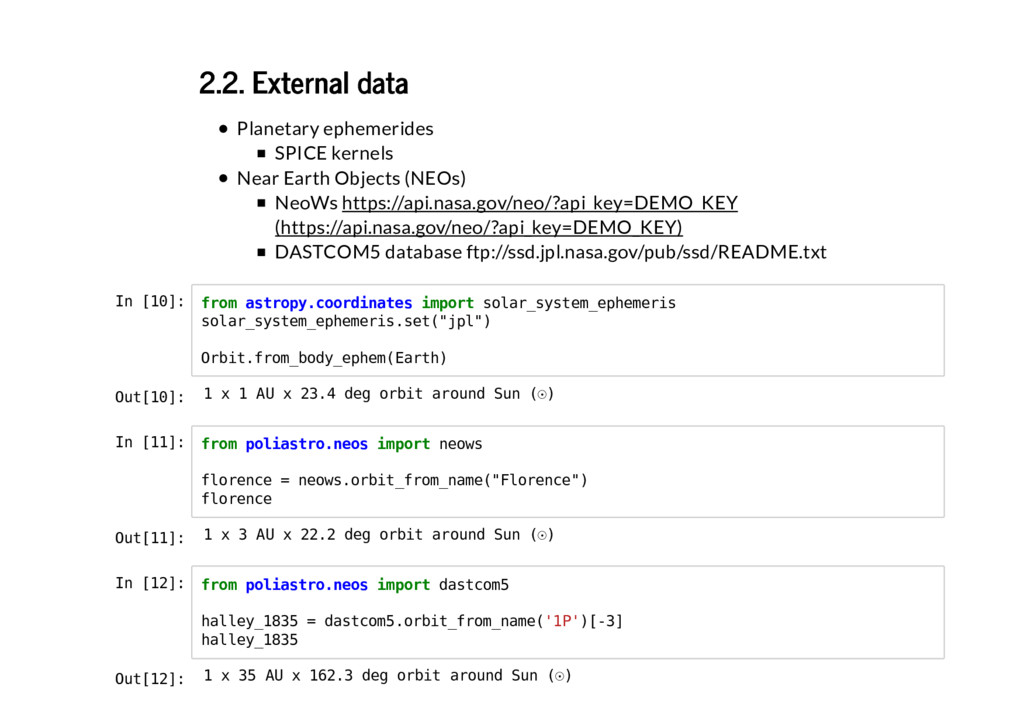
9. 2.2. External data 2.2. External data Planetary ephemerides SPICE kernels Near Earth Objects (NEOs) NeoWs DASTCOM5 database ftp://ssd.jpl.nasa.gov/pub/ssd/README.txt https://api.nasa.gov/neo/?api_key=DEMO_KEY (https://api.nasa.gov/neo/?api_key=DEMO_KEY) In [10]: from astropy.coordinates import solar_system_ephemeris solar_system_ephemeris.set("jpl") Orbit.from_body_ephem(Earth) Out[10]: 1 x 1 AU x 23.4 deg orbit around Sun (☉) In [11]: from poliastro.neos import neows florence = neows.orbit_from_name("Florence") florence Out[11]: 1 x 3 AU x 22.2 deg orbit around Sun (☉) In [12]: from poliastro.neos import dastcom5 halley_1835 = dastcom5.orbit_from_name('1P')[-3] halley_1835 Out[12]: 1 x 35 AU x 162.3 deg orbit around Sun (☉)
10. In [13]: from poliastro.plotting import OrbitPlotter from poliastro.bodies import Mercury, Venus, Earth, Mars frame = OrbitPlotter(num_points=300) # Florence close approach frame.plot(Orbit.from_body_ephem(Earth, epoch=Time("2017-09-01 12:05:50", scale="td b")), label=Earth) for planet in Mercury, Venus, Mars: frame.plot(Orbit.from_body_ephem(planet), label=planet) frame.plot(halley_1835, label='Halley', color='#666666') frame.plot(florence, label='Florence', color='#000000') plt.title("Inner solar system + Florence + Halley") plt.xlim(-.3e9, .3e9) plt.ylim(-.3e9, .3e9) Out[13]: (-300000000.0, 300000000.0)
12. 2.3. Core algorithms 2.3. Core algorithms Analytical propagation, aka Kepler's problem (Battin universal variables approach) Numerical propagation (Cowell's method) Boundary-value problem, aka Lambert's problem (Izzo algorithm with multiple revolution) Orbital maneuvers (Hohmann's transfer, bielliptic transfer)
13. Analytical propagation: In [14]: florence.nu Out[14]: −0.40059292 rad In [15]: florence.propagate(1 * u.day).nu Out[15]: 5.9016222 rad
14. Numerical propagation: In [17]: from poliastro.twobody.propagation import propagate, cowell from poliastro.twobody.decorators import state_from_vector from poliastro.util import norm In [18]: @state_from_vector def accel(t0, ss): v = ss.v.value norm_v = norm(v) return 1e-5 * v / norm_v
15. In [19]: ss Out[19]: 7283 x 10293 km x 153.2 deg orbit around Earth (♁) In [20]: propagate(ss, 3 * u.day, method=cowell, rtol=1e-9, ad=accel, callback=results) Out[20]: 21188 x 24857 km x 153.2 deg orbit around Earth (♁)
16. In [24]: frame = OrbitPlotter3D() frame.set_attractor(Earth) frame.plot_trajectory(results.r) frame.show() Out[24]:
17. Lambert's problem: In [26]: date_launch = Time('2011-11-26 15:02', scale='utc').tdb date_arrival = Time('2012-08-06 05:17', scale='utc').tdb ss_e0 = Orbit.from_body_ephem(Earth, date_launch) ss_mf = Orbit.from_body_ephem(Mars, date_arrival) tof = date_arrival - date_launch (v0, v), = lambert(Sun.k, ss_e0.r, ss_mf.r, tof) In [27]: v0 Out[27]: [−29.291373, 14.532221, 5.4164177] km s In [29]: v Out[29]: [17.615607, − 10.998499, − 4.2080014] km s
18. Orbital maneuvers: In [30]: from poliastro.maneuver import Maneuver In [31]: ss_i = Orbit.circular(Earth, alt=700 * u.km) ss_i Out[31]: 7078 x 7078 km x 0.0 deg orbit around Earth (♁) In [32]: hoh = Maneuver.hohmann(ss_i, 36000 * u.km) hoh.get_total_cost() Out[32]: 3.6173999 km s
19. In [33]: frame = OrbitPlotter() ss_a, ss_f = ss_i.apply_maneuver(hoh, intermediate=True) frame.plot(ss_i, label="Initial orbit") frame.plot(ss_a, label="Transfer orbit") frame.plot(ss_f, label="Final orbit");
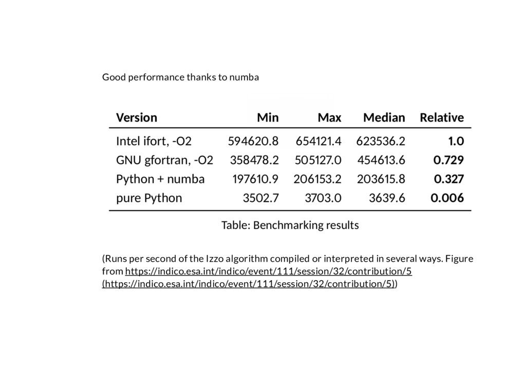
20. Good performance thanks to numba (Runs per second of the Izzo algorithm compiled or interpreted in several ways. Figure from ) https://indico.esa.int/indico/event/111/session/32/contribution/5 (https://indico.esa.int/indico/event/111/session/32/contribution/5)
21. 3. Future work (2 minutes) 3. Future work (2 minutes) Continuous-thrust maneuvers and perturbations: Several optimal or quasi-optimal transfer maneuvers (studied as part of my �nal MSc project ) Solar pressure, atmospheric drag, third body effects... https://github.com/Juanlu001/pfc-uc3m (https://github.com/Juanlu001/pfc-uc3m) Improvements on propagation: Support for events (pericenter and apocenter passage, eclipses, custom events) Better convergence Storage of intermediate results (plotting, analysis) Better validation: So far, results from textbook assignments and scholarly papers: scarce and often not available in full precision Next step: validate against SPICE
22. ...And, perhaps more importantly, attract contributors!
23. 4. Conclusions 4. Conclusions poliastro offers an attractive, easy to use API while being "fast enough" Lots of functionality provided by a strong ecosystem of packages Interactive visualization is useful in preliminary analysis There is some work to do to add more features and improve stability We would love to have you as a contributor!
24. Per Python ad astra ➭ ✉ https://www.linkedin.com/in/juanluiscanor (https://www.linkedin.com /in/juanluiscanor) hello@juanlu.space (mailto:hello@juanlu.space) https://github.com/poliastro/oscw2017-talk (https://github.com/poliastro /oscw2017-talk)