On the Flatness of Loss Surface for Two-layered ReLU Networks

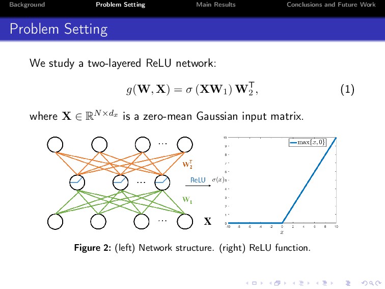
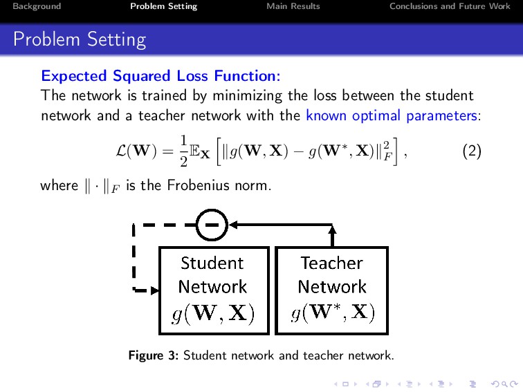
Deep learning has achieved unprecedented practical success in many applications. Despite its empirical success, however, the theoretical understanding of deep neural networks still remains a major open problem. In this paper, we explore properties of two-layered ReLU networks. For simplicity, we assume that the optimal model parameters (also called ground-truth parameters) are known. We then assume that a network receives Gaussian input and is trained by minimizing the expected squared loss between the prediction function of the network and a target function. To conduct the analysis, we propose a normal equation for critical points, and study the invariances under three kinds of transformations, namely, scale transformation, rotation transformation and perturbation transformation. We prove that these transformations can keep the loss of a critical point invariant, thus can incur at regions. Consequently, how to escape from at regions is vital in training neural networks.

Transcript

1. Background Problem Setting Main Results Conclusions and Future Work On the Flatness of Loss Surface for Two-layered ReLU Networks Jiezhang Cao1, Qingyao Wu1, Yuguang Yan1, Li Wang2, Mingkui Tan1 1School of Software Engineering, South China University of Technology 2Department of Mathematics, University of Texas at Arlington November 17, 2017
2. Background Problem Setting Main Results Conclusions and Future Work Outline 1 Background 2 Problem Setting 3 Main Results 4 Conclusions and Future Work
3. Background Problem Setting Main Results Conclusions and Future Work Deep Learning Figure 1: Image recognition
4. Background Problem Setting Main Results Conclusions and Future Work Notations We will use the following notations: Let σ(M) = max(0, M) : Rm×n → Rm×n be the element-wise ReLU function of a matrix M ∈ Rm×n. Let vec(M) ∈ Rmn be a vectorization of a matrix M ∈ Rm×n. Let Dvec(M) f(·) = ∂f(·) ∂ vec(M) be the partial derivative of f(·) with respect to vec (M).
5. Background Problem Setting Main Results Conclusions and Future Work Problem Setting We study a two-layered ReLU network: g(W, X) = σ (XW1) WT 2 , (1) where X ∈ RN×dx is a zero-mean Gaussian input matrix. Figure 2: (left) Network structure. (right) ReLU function.
6. Background Problem Setting Main Results Conclusions and Future Work Problem Setting Expected Squared Loss Function: The network is trained by minimizing the loss between the student network and a teacher network with the known optimal parameters: L(W) = 1 2EX g(W, X) − g(W∗, X) 2 F , (2) where · F is the Frobenius norm. Figure 3: Student network and teacher network.
7. Background Problem Setting Main Results Conclusions and Future Work What does the loss surface look like?
8. Background Problem Setting Main Results Conclusions and Future Work Two key questions: Does the flatness exist? The answer is YES! What causes the flatness? Why Flat?
9. Background Problem Setting Main Results Conclusions and Future Work Main Contributions Our main contributions: We study the flatness of loss surface for general two-layered ReLU networks without the fixed-weights for the last layer. We provide a normal equation for the loss function to understand the behaviors of critical points and the loss function. We consider three kinds of transformations and explore the invariance of the loss function.
10. Background Problem Setting Main Results Conclusions and Future Work Important Definitions Flatness of Critical Point Given > 0, a critical point W, and a loss L(W), we define C(L, W, ) as the largest connected set containing W, such that ∀ W ∈ C(L, W, ), |L(W) − L(W )| < . Define the -flatness as the volume of C(L, W, ). Every point in the nearby region should have a small loss difference. Figure 4: Flatness of a critical point (e.g., local minima).
11. Background Problem Setting Main Results Conclusions and Future Work Important Definitions Isolated Critical Point Given a largest connected set C(L, W, ), a critical point W is isolated if W is not the only critical point. Otherwise it is non-isolated. Figure 5: Isolated critical point (e.g., local minima).
12. Background Problem Setting Main Results Conclusions and Future Work Main Results Recall that the expected squared loss function is L(W) = 1 2EX g(W, X) − g(W∗, X) 2 F . Normal Equation: We set the expectation of the partial derivative of L(W) to 0, 0 = E Dvec(W1) L(W) T = N 2π k (Ak − A∗ k ) W2Pk, (3) 0 = E Dvec(W2) L(W) T = N 2π k PkWT 1 (Ak − A∗ k ) . (4)
13. Background Problem Setting Main Results Conclusions and Future Work Main Results Invariance under Scale Transformation Theorem 1 [Scale invariance] If W = {W1 , W2 } is a critical point satisfying Eqns. (3) and (4), then for any α > 0, ˆ W = Tα (W) = {αW1 , α−1W2 } is also a critical point, and L(W) = L( ˆ W). Tα does not affect the prediction function and the loss function. Proposition 2 Given a two-layered ReLU network, it follows that a critical point W = 0 is non-isolated, and ∀ > 0, C(L, W, ) has an infinite volume. Around every critical point, there exists an infinitely large region with the approximately constant losses.
14. Background Problem Setting Main Results Conclusions and Future Work Main Results Invariance under Rotation Transformation Theorem 2 [Rotation Invariance] If W = {W1 , W2 } is a critical point satisfying Eqns. (3) and (4), for any orthogonal mapping matrices R1 and R2 with R1 |Π∗ 1 = Idx and R2 |Π∗ 2 = Idy such that R1 W∗ 1 = W∗ 1 and R2 W∗ 2 = W∗ 2 , respectively, then ¯ W = {R1 W1 , W2 R2 } is also a critical point. Figure 6: The Mexican hat example. Rotation transforms a local minima to a different one.
15. Background Problem Setting Main Results Conclusions and Future Work Main Results Invariance under Rotation Transformation Principal Hyperplane Define Π∗ 1 and Π∗ 2 as Principal Hyperplanes spanned by the ground-truth weight vectors W∗ 1 = [w∗ 1 (1), . . . , w∗ d 1 (1)] and W∗ 2 = w∗ 1 (2), . . . , w∗ d 1 (2) , respectively. w(i) j d1 j=1 is said to be in-plane, if all w(i) j ∈ Π∗, where i ∈ {1, 2}; Otherwise, it is out-of-plane. Theorem 3 Given dx ≥ d1 + 2 or dy ≥ d1 + 2, if a critical point W satisfying Eqns. (3) and (4) is out-of-plane, then it is non-isolated and lies in a manifold. For ∀ > 0, C(L, W, ) has a large volume -flatness in this manifold. The out-of-plane critical points lie on a manifold.
16. Background Problem Setting Main Results Conclusions and Future Work Main Results Invariance under Rotation Transformation Figure 7: Out-of-plane critical points lie in a manifold.
17. Background Problem Setting Main Results Conclusions and Future Work Main Results Invariance under Perturbation Transformation Perturbation Transformation Given two points W and ¯ W, we define a perturbation transformation on a straight line as: Pµ (W, ¯ W) = W + µ( ¯ W − W), µ > 0. Figure 8: Perturb between two points.
18. Background Problem Setting Main Results Conclusions and Future Work Main Results Invariance under Perturbation Transformation Theorem 5 [Perturbation Invariance] Given a fixed weight matrix W1 , if W = {W1 , W2 } is a critical point satisfying Eq. (4), then there exists a perturbation of W2 , such that ˜ W = {W1 , ˜ W2 } is also a critical point and is non-isolated. There exists a flat region with the approximately constant losses. Theorem 6 [A Special Case without Perturbation Invariance] Let W = {W1 , W2 } be a critical point satisfying Eqns. (3) and (4), for any orthogonal mapping pair R1 and R2 with R1 |Π∗ 1 = Idx and R2 |Π∗ 2 = Idy , if ¯ W1 = R1 W1 and ¯ W2 = R2 W2 , then ˜ W = Pµ (W, ¯ W) = { ˜ W1 , ˜ W2 } cannot be a critical point. For a special case, there does not exist perturbation invariance for another critical point.
19. Background Problem Setting Main Results Conclusions and Future Work Main Results Invariance under Perturbation Transformation Figure 9: (left) Perturbation Invariance. (right) A Special Case without Perturbation Invariance.
20. Background Problem Setting Main Results Conclusions and Future Work Conclusions Our conclusions: Three kinds of transformations keep the losses invariant. The flat loss surface can be formed by connected critical points.
21. Background Problem Setting Main Results Conclusions and Future Work Future Work Our future work: We will generalize the Gaussian distribution to a general distribution. We will study a multi-layed ReLU network. We will address the flatness issue in training the neural networks.
22. Background Problem Setting Main Results Conclusions and Future Work Thank you