Carlisle Rainey Assistant Professor Texas A&M University [email protected] Holger Kern Assistant Professor Florida State University [email protected] paper, data, and code at carlislerainey.com/talk
Carlisle Rainey Assistant Professor Texas A&M University [email protected] Holger Kern Assistant Professor Florida State University [email protected] paper, data, and code at carlislerainey.com/talk
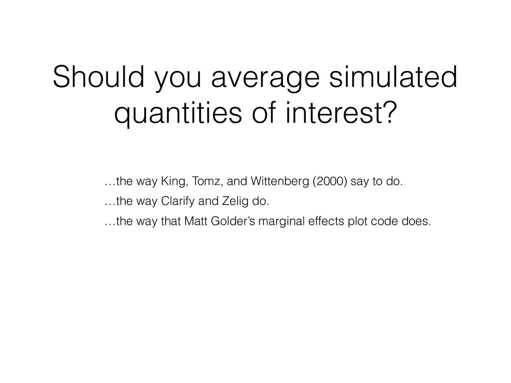
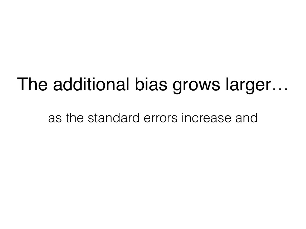
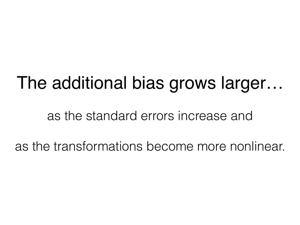
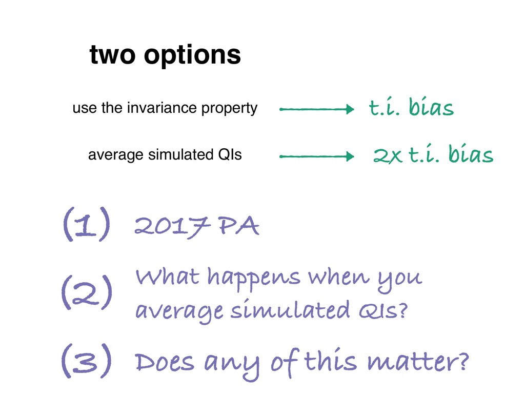
…the way Clarify and Zelig do. …the way that Matt Golder’s marginal effects plot code does. …the way that Hanmer and Kalkan’s (2013) code does. Should you average simulated quantities of interest?
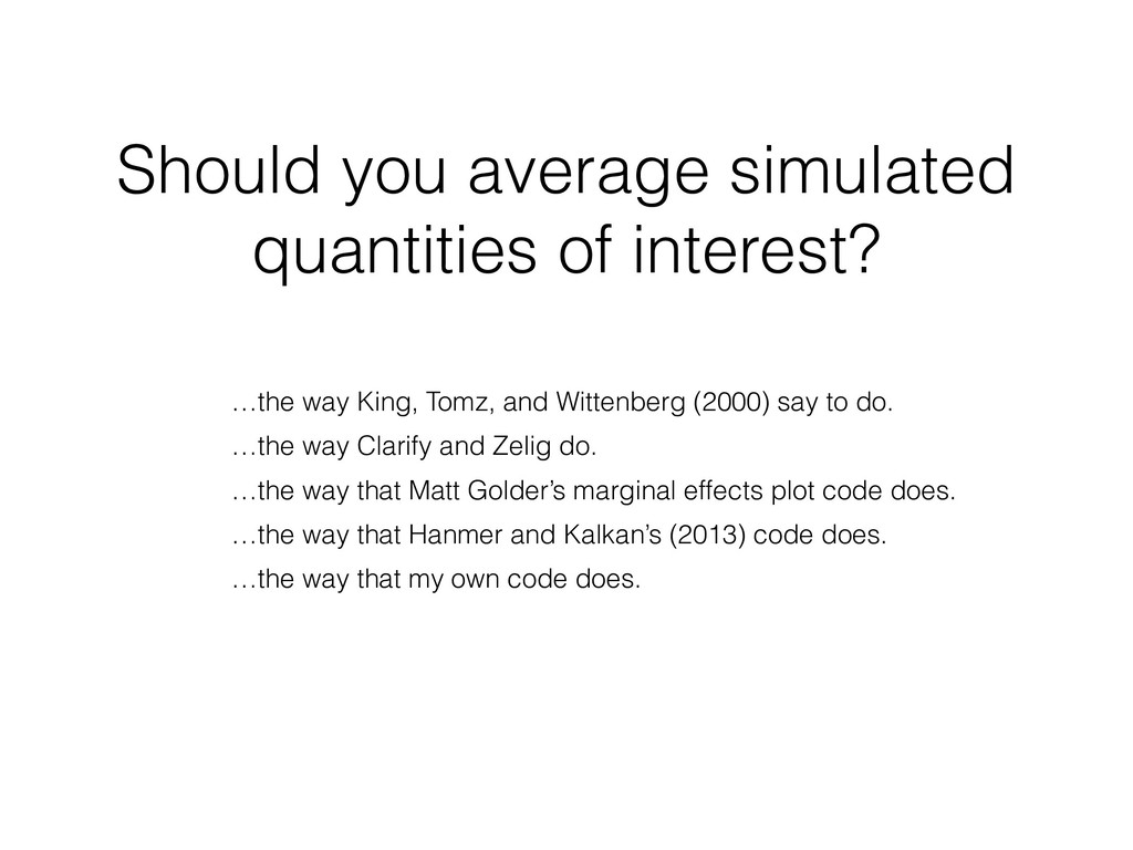
…the way Clarify and Zelig do. …the way that Matt Golder’s marginal effects plot code does. …the way that Hanmer and Kalkan’s (2013) code does. …the way that my own code does. Should you average simulated quantities of interest?
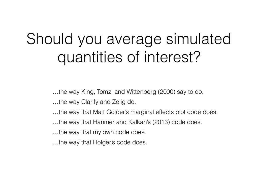
…the way Clarify and Zelig do. …the way that Matt Golder’s marginal effects plot code does. …the way that Hanmer and Kalkan’s (2013) code does. …the way that my own code does. …the way that Holger’s code does. Should you average simulated quantities of interest?
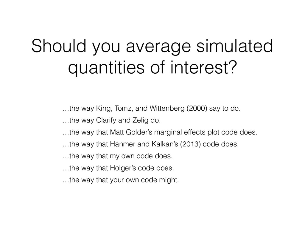
…the way Clarify and Zelig do. …the way that Matt Golder’s marginal effects plot code does. …the way that Hanmer and Kalkan’s (2013) code does. …the way that my own code does. …the way that Holger’s code does. …the way that your own code might. Should you average simulated quantities of interest?
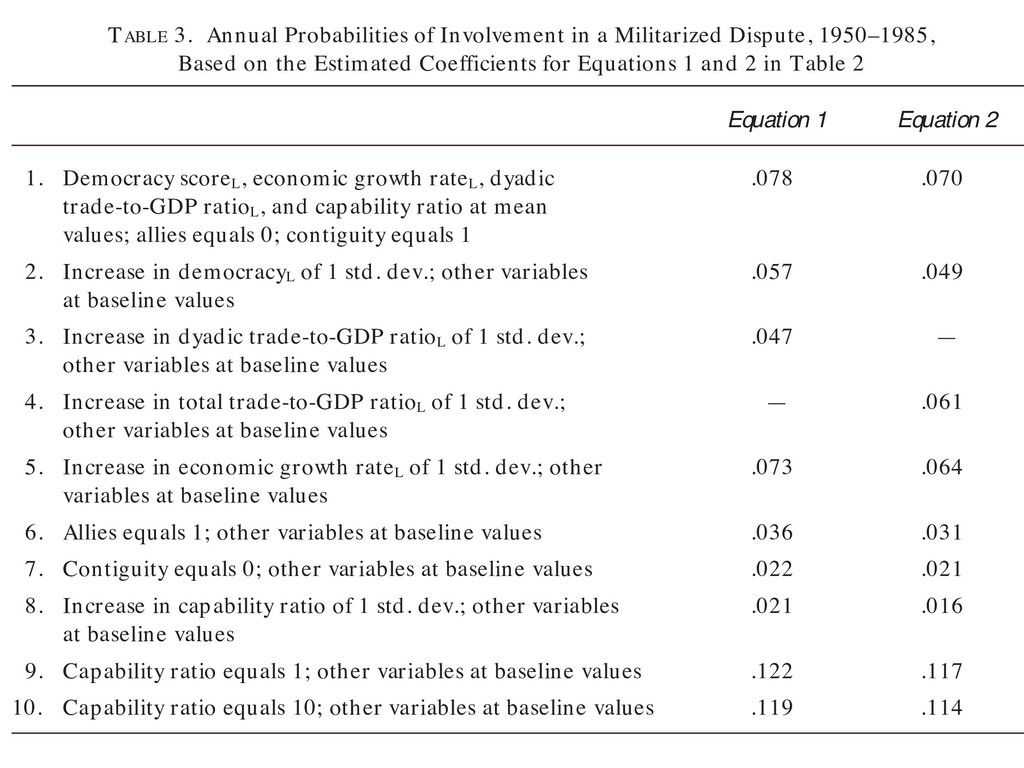
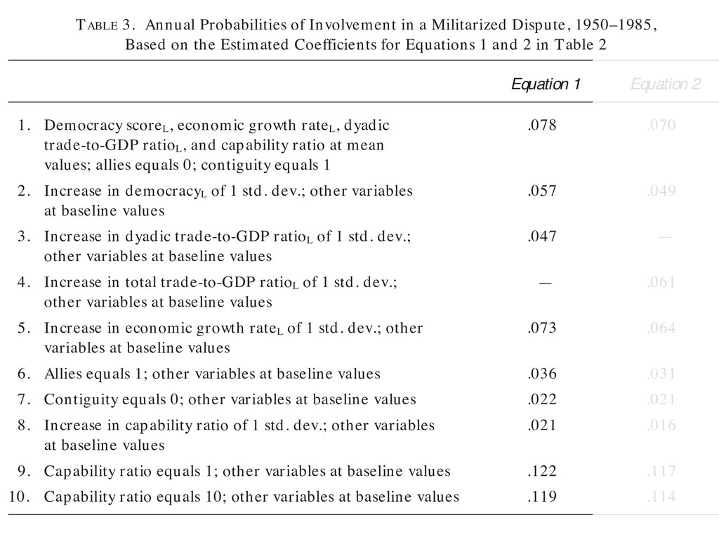
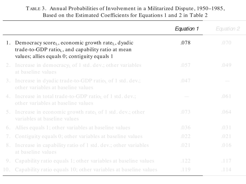
1950–1985, Based on the Estimated Coefficients for Equations 1 and 2 in Table 2 Equation 1 Equation 2 1. Democracy scoreL , economic growth rateL , dyadic .078 .070 trade-to-GDP ratioL , and capability ratio at mean values; allies equals 0; contiguity equals 1 2. Increase in democracyL of 1 std. dev.; other variables .057 .049 at baseline values 3. Increase in dyadic trade-to-GDP ratioL of 1 std. dev.; .047 — other variables at baseline values 4. Increase in total trade-to-GDP ratioL of 1 std. dev.; — .061 other variables at baseline values 5. Increase in economic growth rateL of 1 std. dev.; other .073 .064 variables at baseline values 6. Allies equals 1; other variables at baseline values .036 .031 7. Contiguity equals 0; other variables at baseline values .022 .021 8. Increase in capability ratio of 1 std. dev.; other variables .021 .016 at baseline values 9. Capability ratio equals 1; other variables at baseline values .122 .117 10. Capability ratio equals 10; other variables at baseline values .119 .114
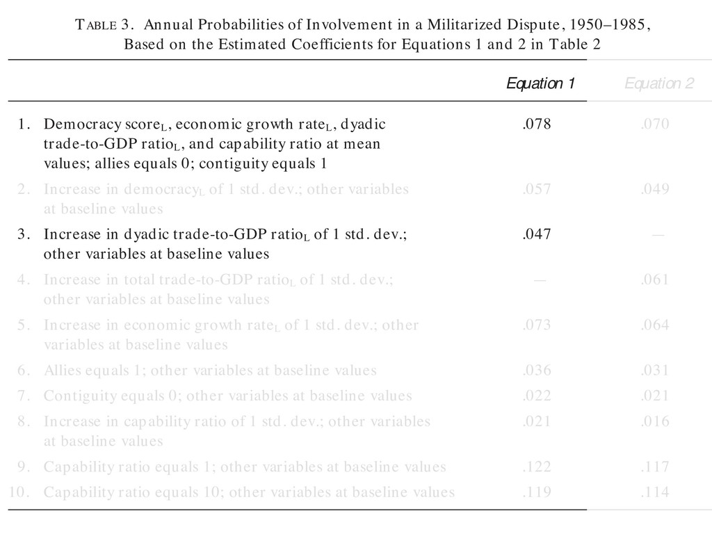
1950–1985, Based on the Estimated Coefficients for Equations 1 and 2 in Table 2 Equation 1 Equation 2 1. Democracy scoreL , economic growth rateL , dyadic .078 .070 trade-to-GDP ratioL , and capability ratio at mean values; allies equals 0; contiguity equals 1 2. Increase in democracyL of 1 std. dev.; other variables .057 .049 at baseline values 3. Increase in dyadic trade-to-GDP ratioL of 1 std. dev.; .047 — other variables at baseline values 4. Increase in total trade-to-GDP ratioL of 1 std. dev.; — .061 other variables at baseline values 5. Increase in economic growth rateL of 1 std. dev.; other .073 .064 variables at baseline values 6. Allies equals 1; other variables at baseline values .036 .031 7. Contiguity equals 0; other variables at baseline values .022 .021 8. Increase in capability ratio of 1 std. dev.; other variables .021 .016 at baseline values 9. Capability ratio equals 1; other variables at baseline values .122 .117 10. Capability ratio equals 10; other variables at baseline values .119 .114
1950–1985, Based on the Estimated Coefficients for Equations 1 and 2 in Table 2 Equation 1 Equation 2 1. Democracy scoreL , economic growth rateL , dyadic .078 .070 trade-to-GDP ratioL , and capability ratio at mean values; allies equals 0; contiguity equals 1 2. Increase in democracyL of 1 std. dev.; other variables .057 .049 at baseline values 3. Increase in dyadic trade-to-GDP ratioL of 1 std. dev.; .047 — other variables at baseline values 4. Increase in total trade-to-GDP ratioL of 1 std. dev.; — .061 other variables at baseline values 5. Increase in economic growth rateL of 1 std. dev.; other .073 .064 variables at baseline values 6. Allies equals 1; other variables at baseline values .036 .031 7. Contiguity equals 0; other variables at baseline values .022 .021 8. Increase in capability ratio of 1 std. dev.; other variables .021 .016 at baseline values 9. Capability ratio equals 1; other variables at baseline values .122 .117 10. Capability ratio equals 10; other variables at baseline values .119 .114
1950–1985, Based on the Estimated Coefficients for Equations 1 and 2 in Table 2 Equation 1 Equation 2 1. Democracy scoreL , economic growth rateL , dyadic .078 .070 trade-to-GDP ratioL , and capability ratio at mean values; allies equals 0; contiguity equals 1 2. Increase in democracyL of 1 std. dev.; other variables .057 .049 at baseline values 3. Increase in dyadic trade-to-GDP ratioL of 1 std. dev.; .047 — other variables at baseline values 4. Increase in total trade-to-GDP ratioL of 1 std. dev.; — .061 other variables at baseline values 5. Increase in economic growth rateL of 1 std. dev.; other .073 .064 variables at baseline values 6. Allies equals 1; other variables at baseline values .036 .031 7. Contiguity equals 0; other variables at baseline values .022 .021 8. Increase in capability ratio of 1 std. dev.; other variables .021 .016 at baseline values 9. Capability ratio equals 1; other variables at baseline values .122 .117 10. Capability ratio equals 10; other variables at baseline values .119 .114
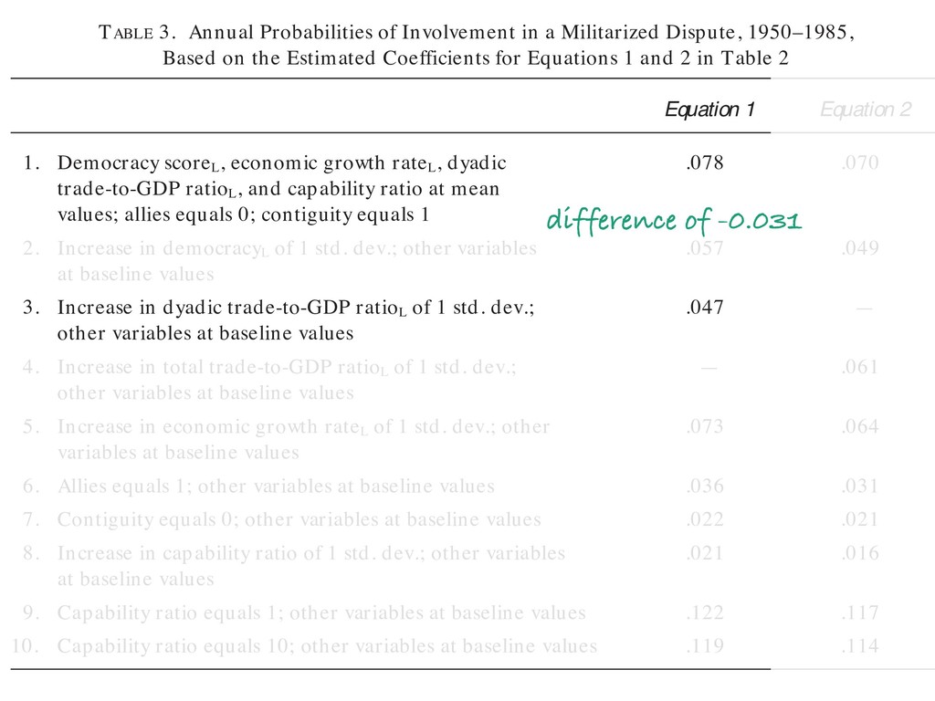
1950–1985, Based on the Estimated Coefficients for Equations 1 and 2 in Table 2 Equation 1 Equation 2 1. Democracy scoreL , economic growth rateL , dyadic .078 .070 trade-to-GDP ratioL , and capability ratio at mean values; allies equals 0; contiguity equals 1 2. Increase in democracyL of 1 std. dev.; other variables .057 .049 at baseline values 3. Increase in dyadic trade-to-GDP ratioL of 1 std. dev.; .047 — other variables at baseline values 4. Increase in total trade-to-GDP ratioL of 1 std. dev.; — .061 other variables at baseline values 5. Increase in economic growth rateL of 1 std. dev.; other .073 .064 variables at baseline values 6. Allies equals 1; other variables at baseline values .036 .031 7. Contiguity equals 0; other variables at baseline values .022 .021 8. Increase in capability ratio of 1 std. dev.; other variables .021 .016 at baseline values 9. Capability ratio equals 1; other variables at baseline values .122 .117 10. Capability ratio equals 10; other variables at baseline values .119 .114 difference of -0.031
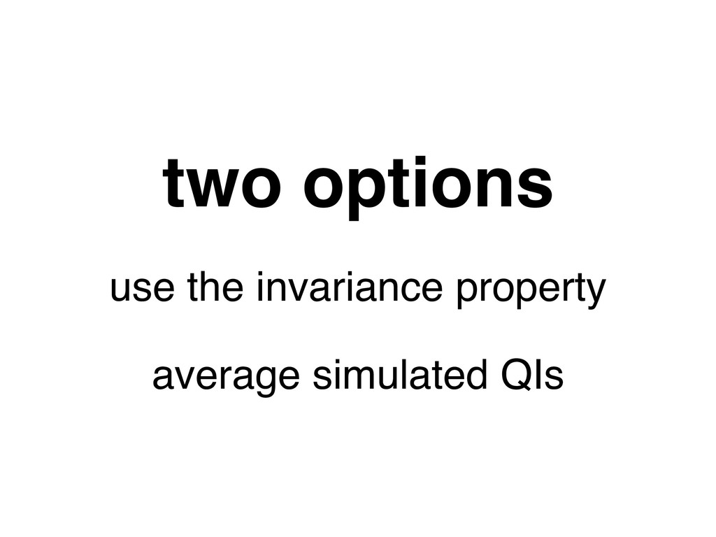
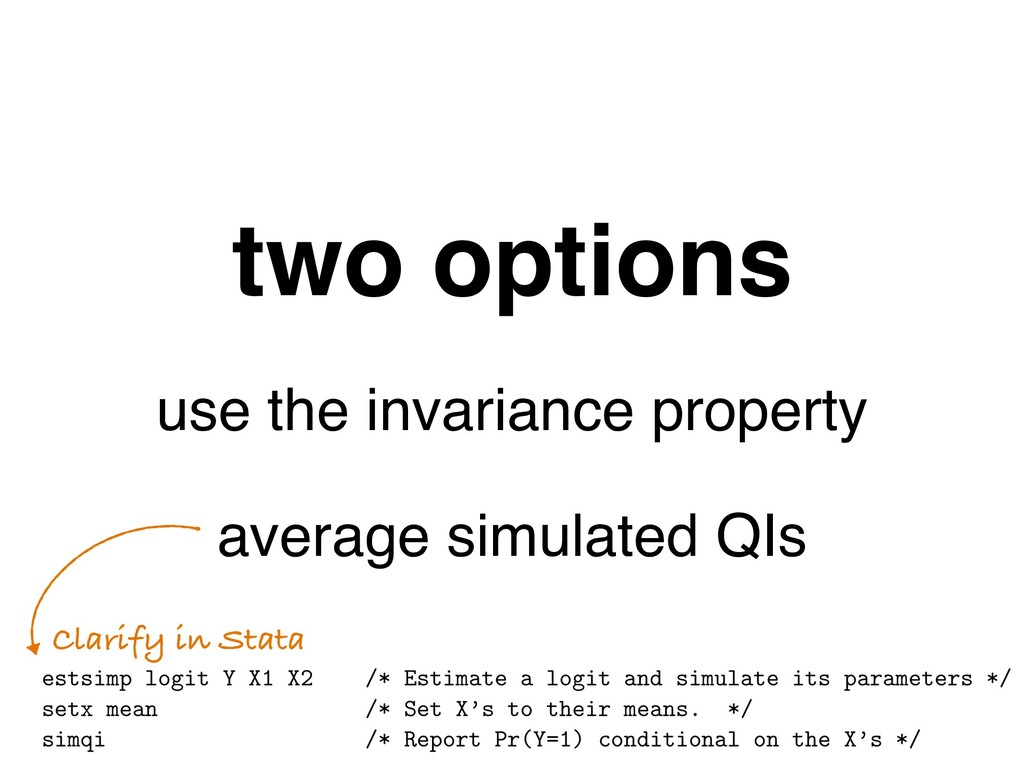
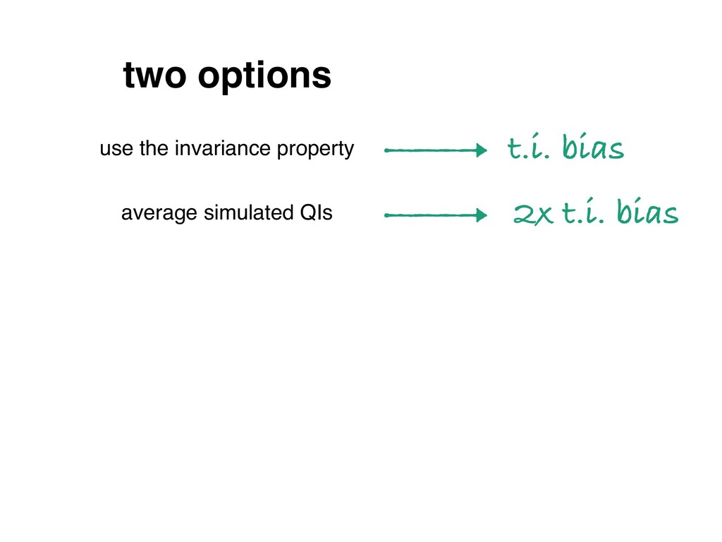
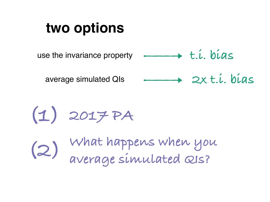
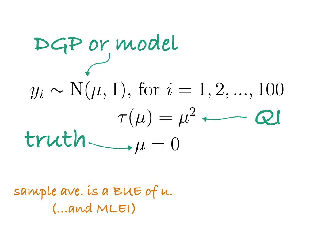
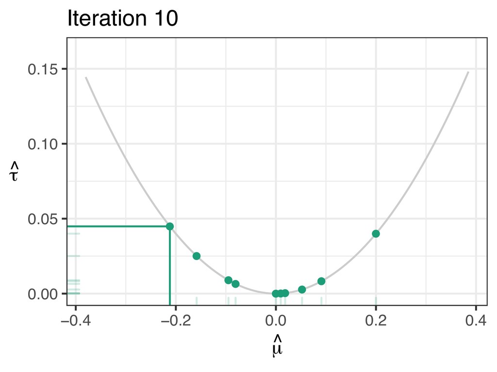
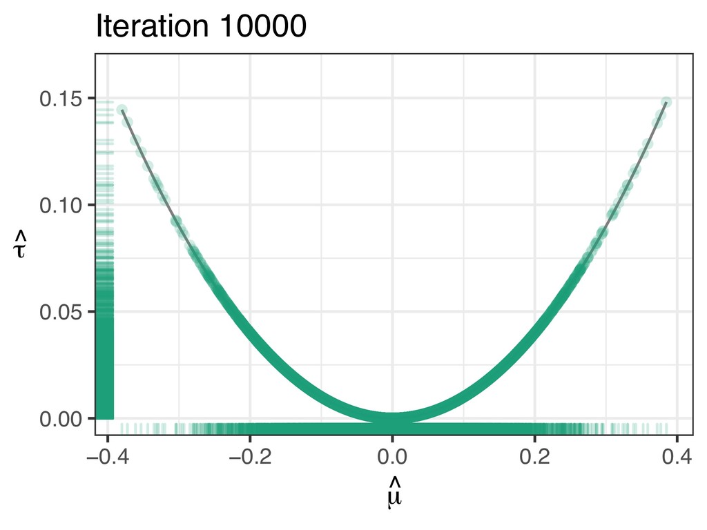
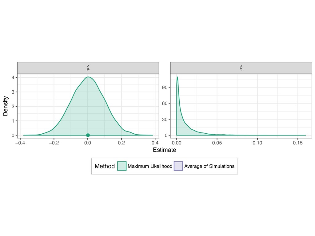
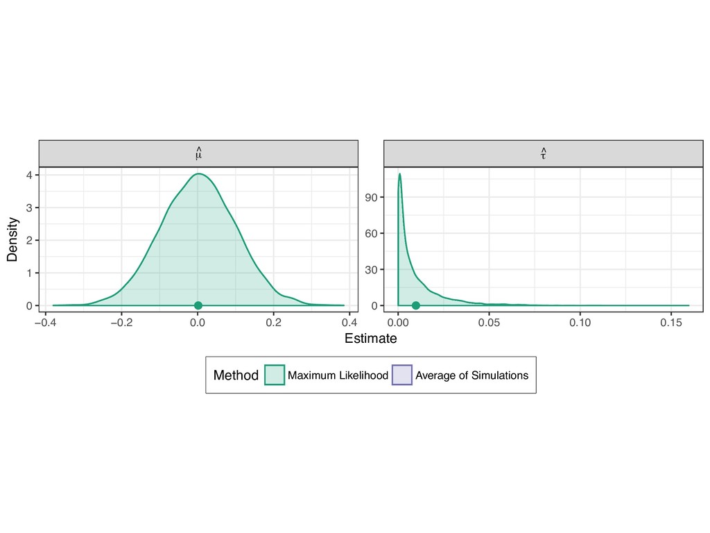
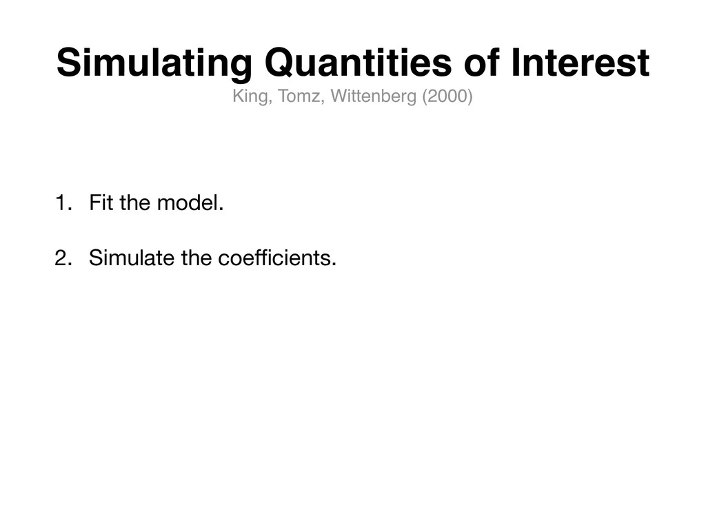
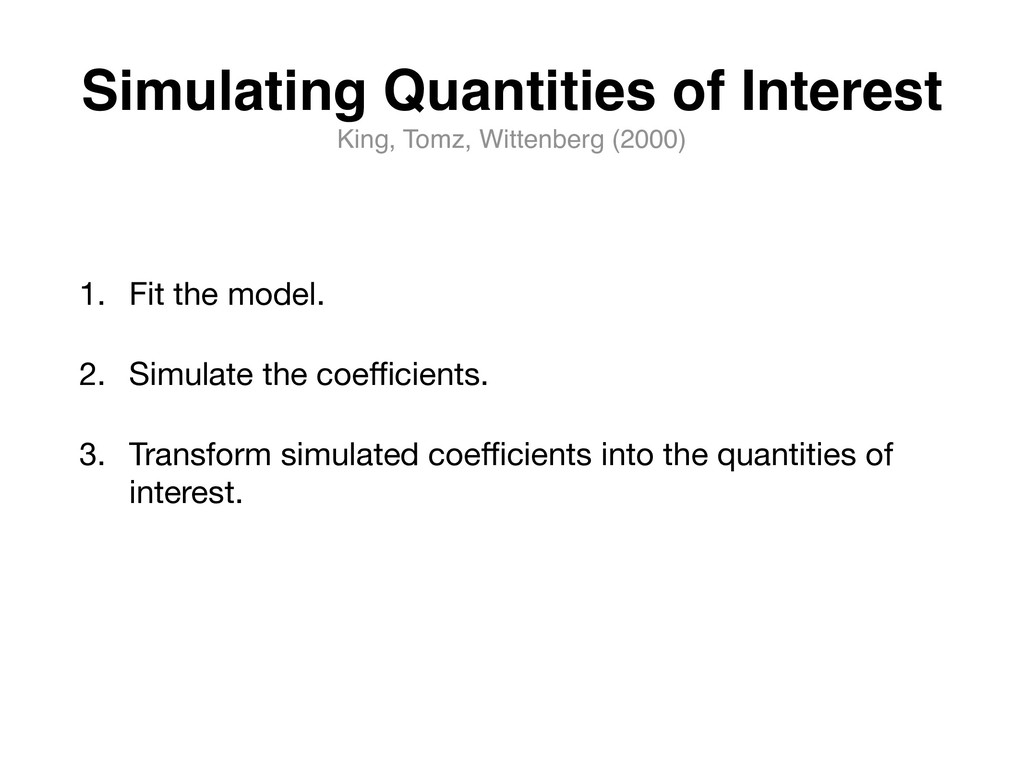
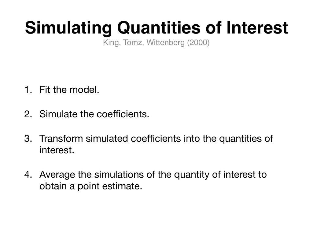
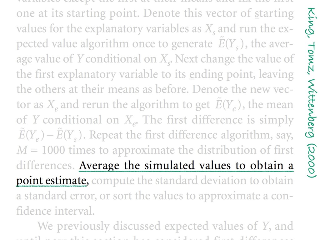
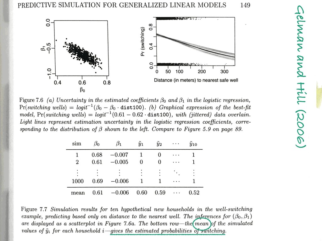
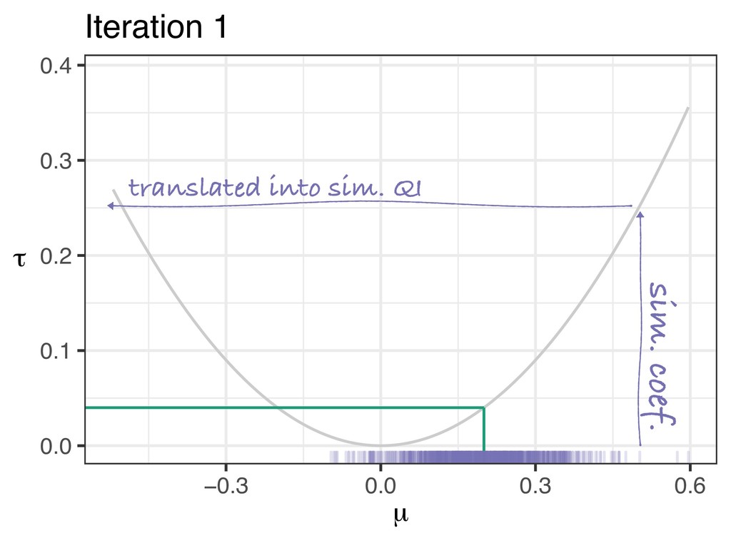
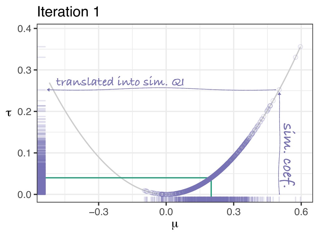
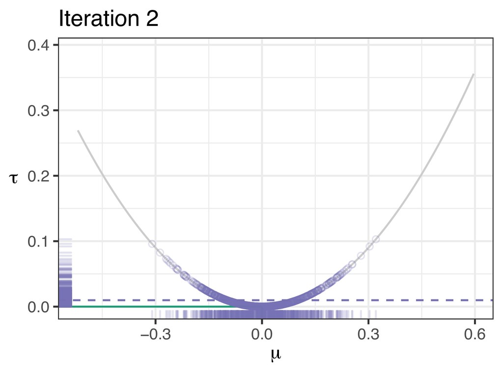
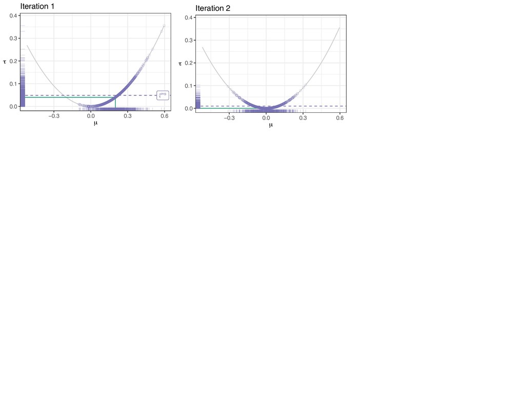
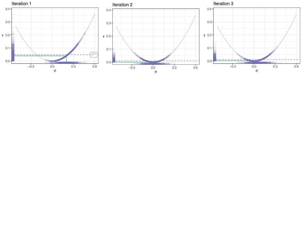
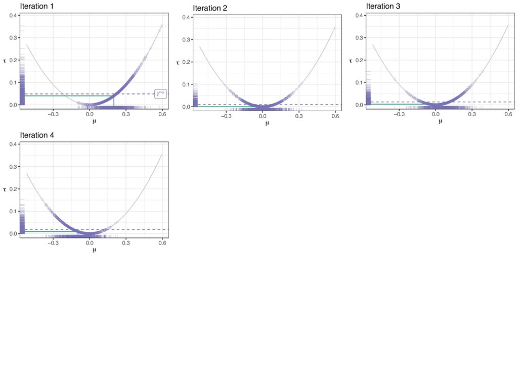
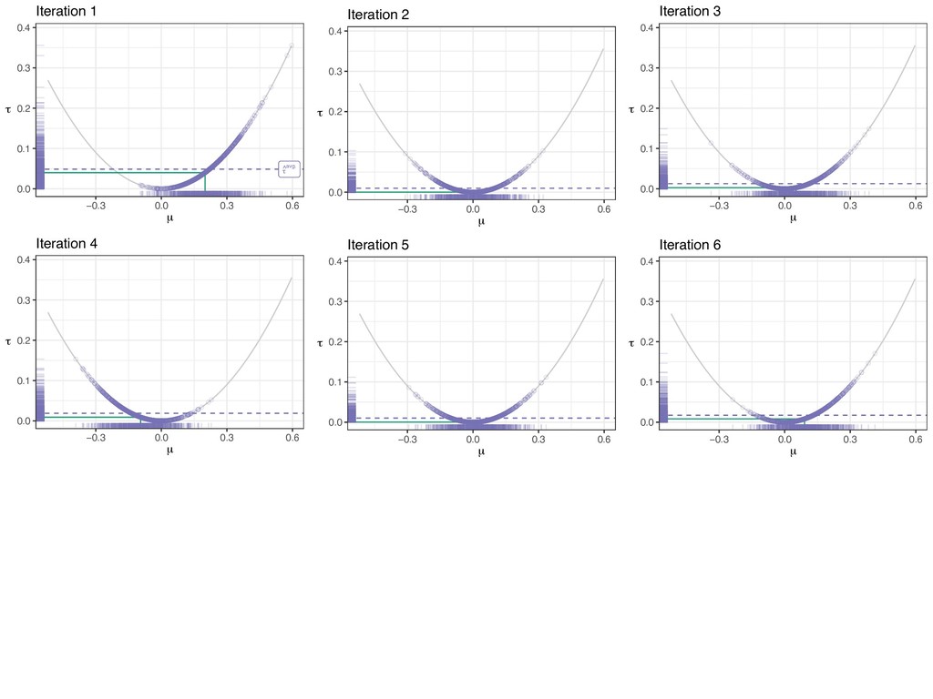
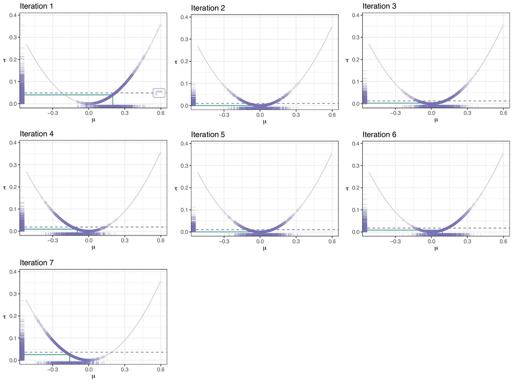
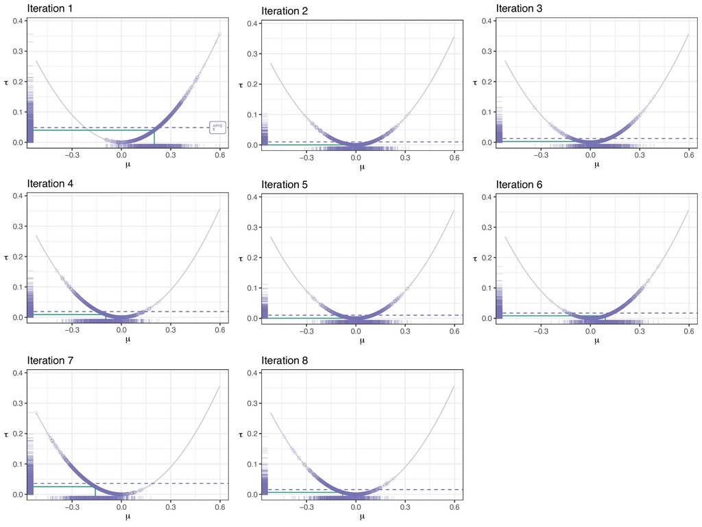
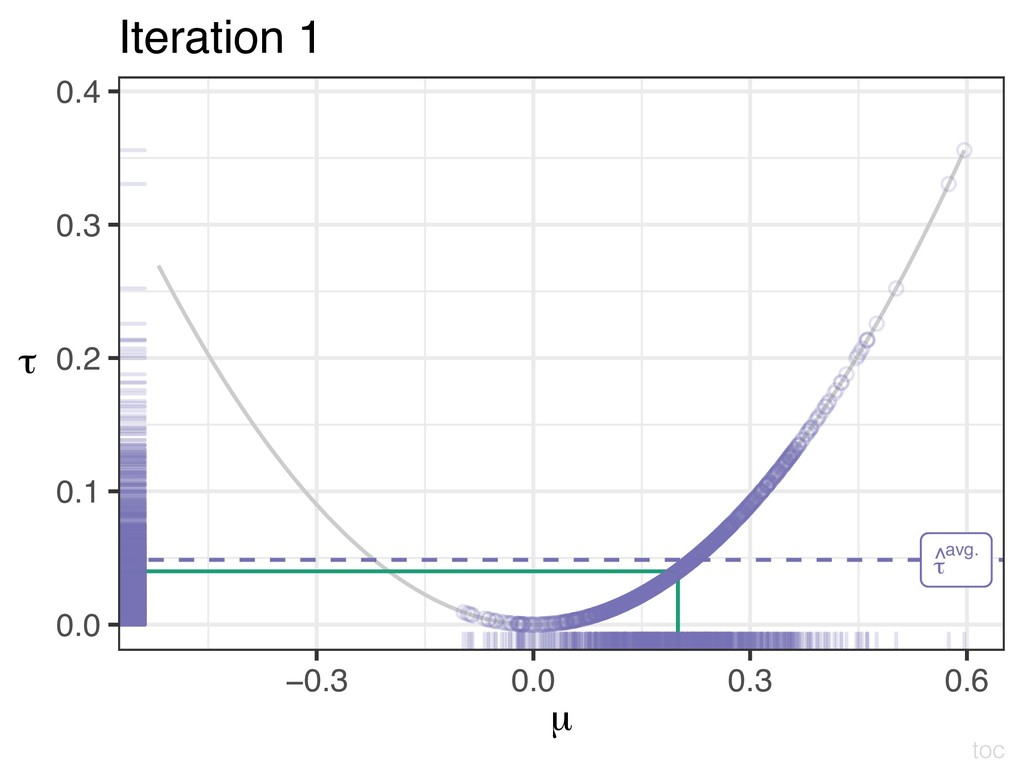
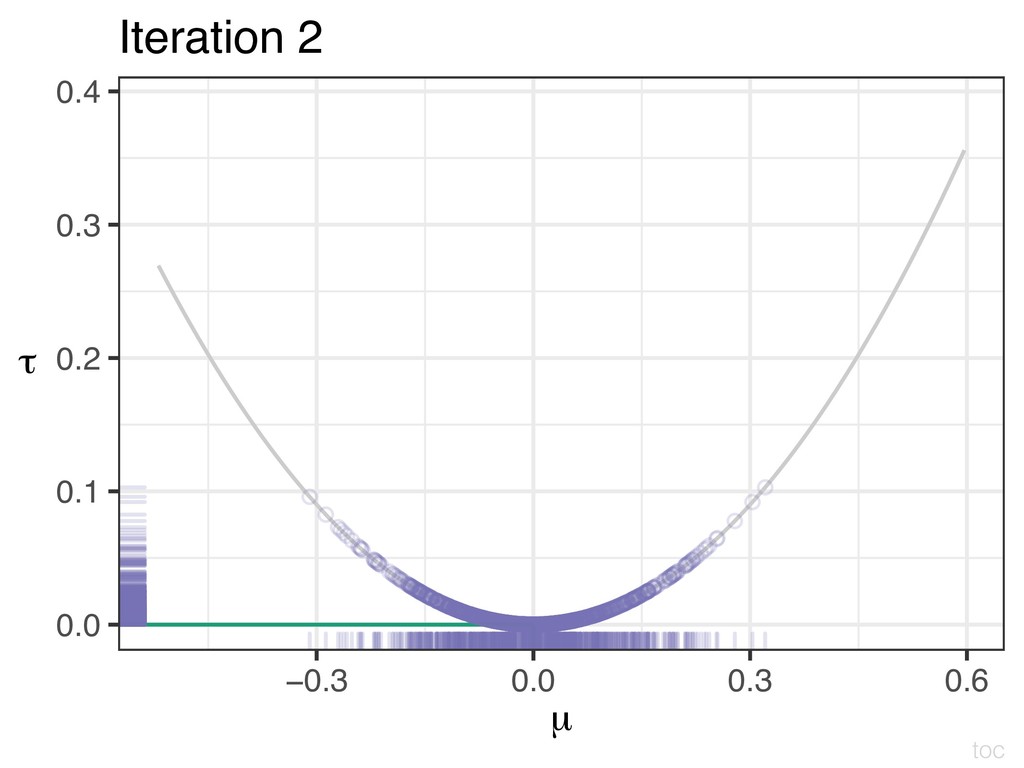
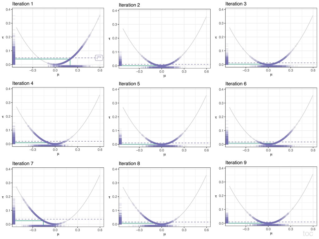
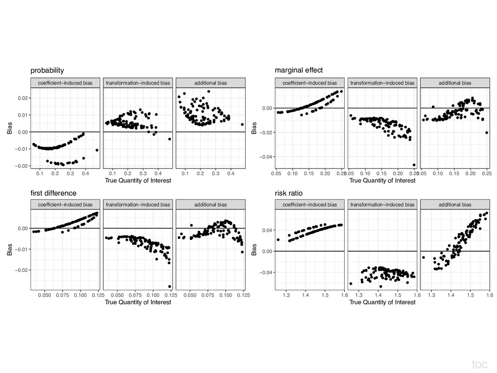
the model. 2. Simulate the coefficients. 3. Transform simulated coefficients into the quantities of interest. 4. Average the simulations of the quantity of interest to obtain a point estimate.
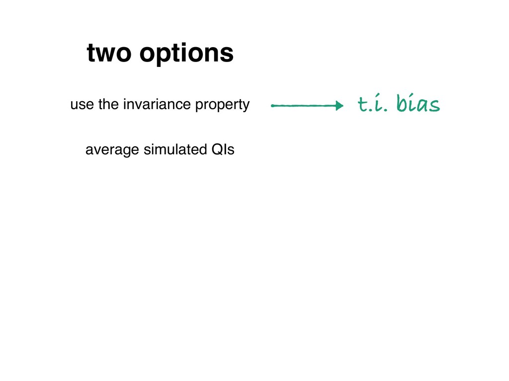
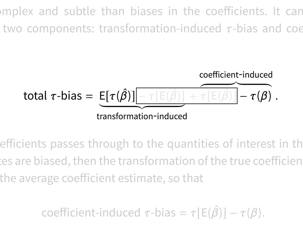
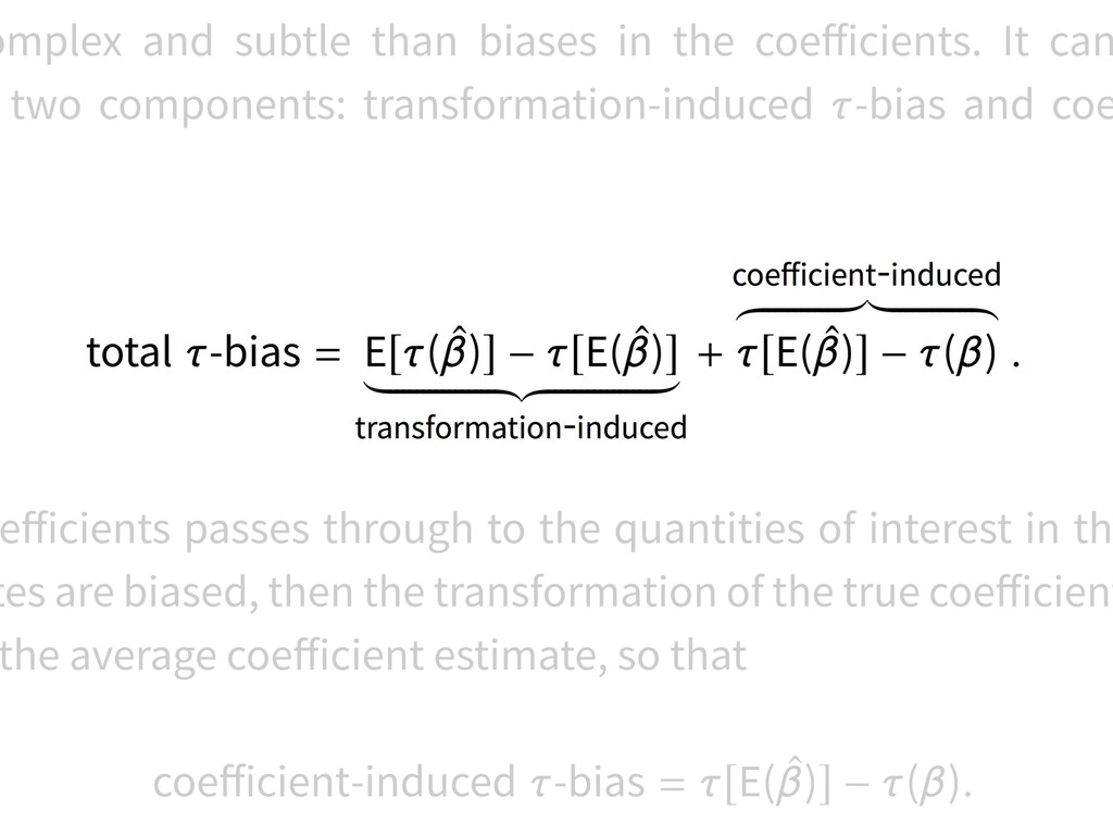
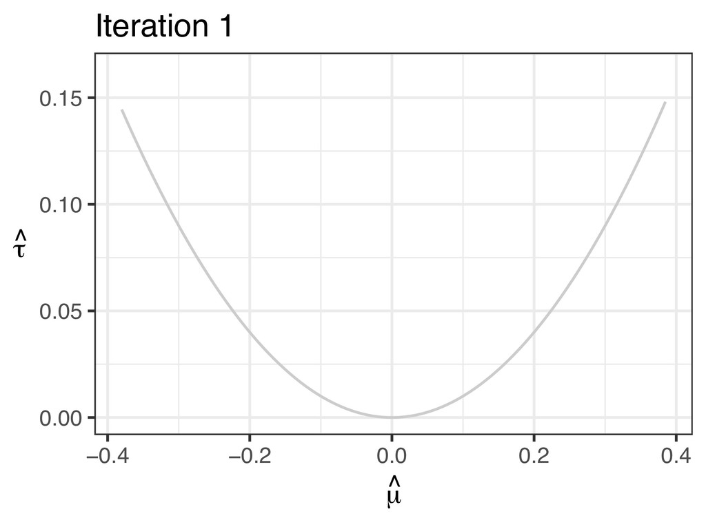
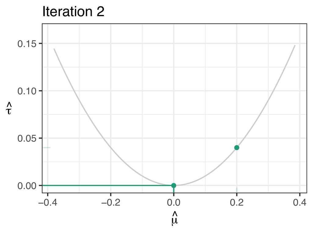
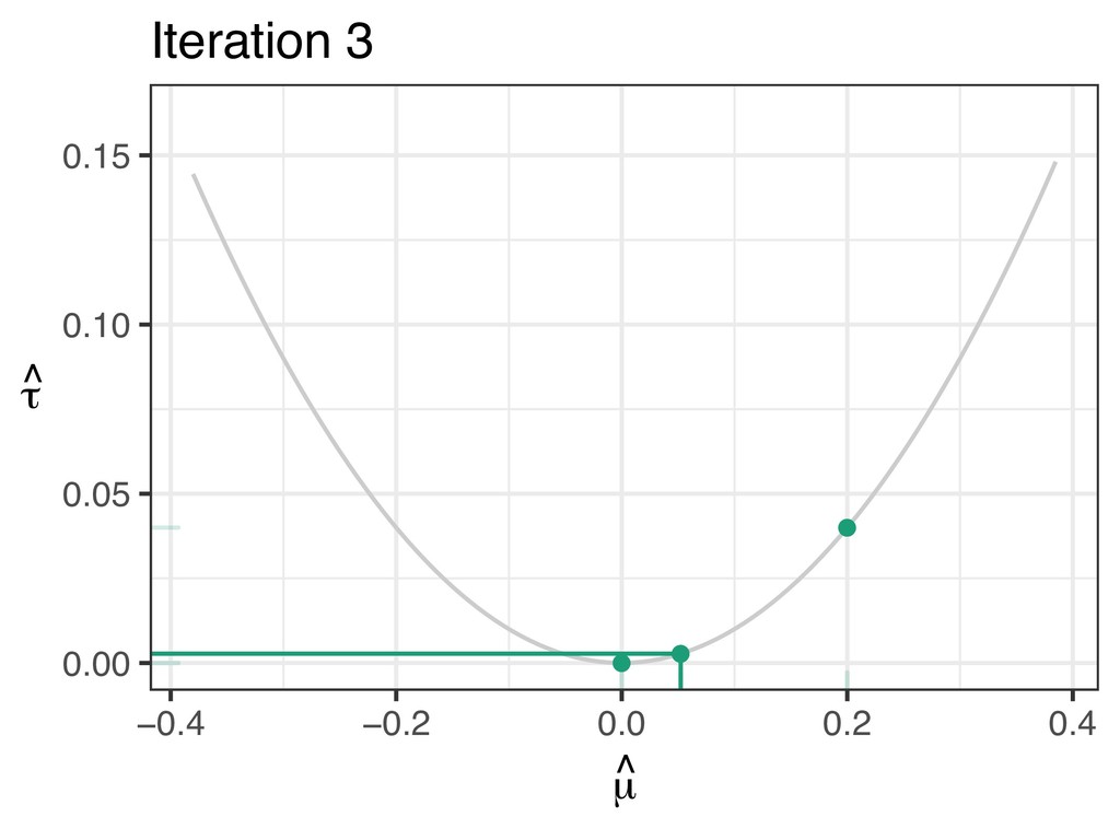
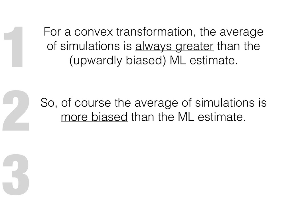
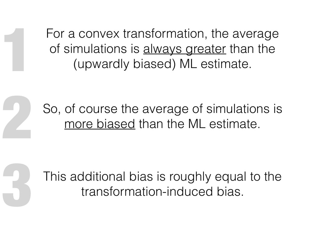
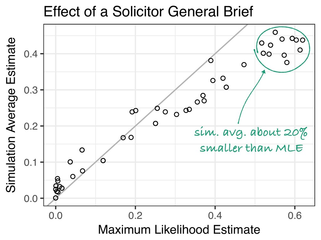
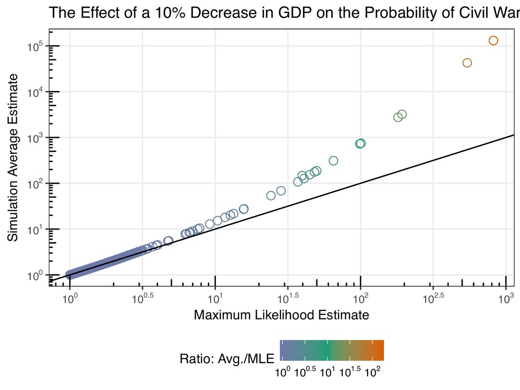
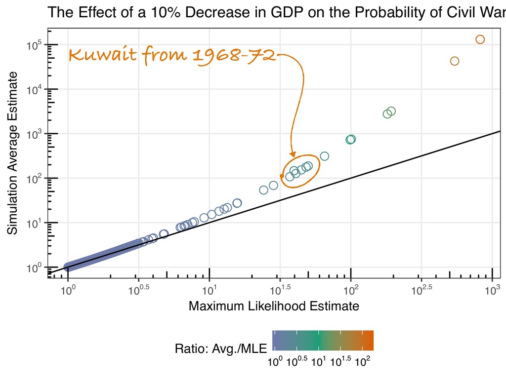
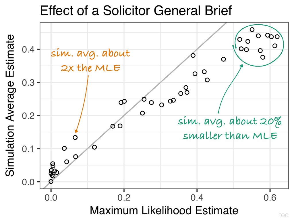
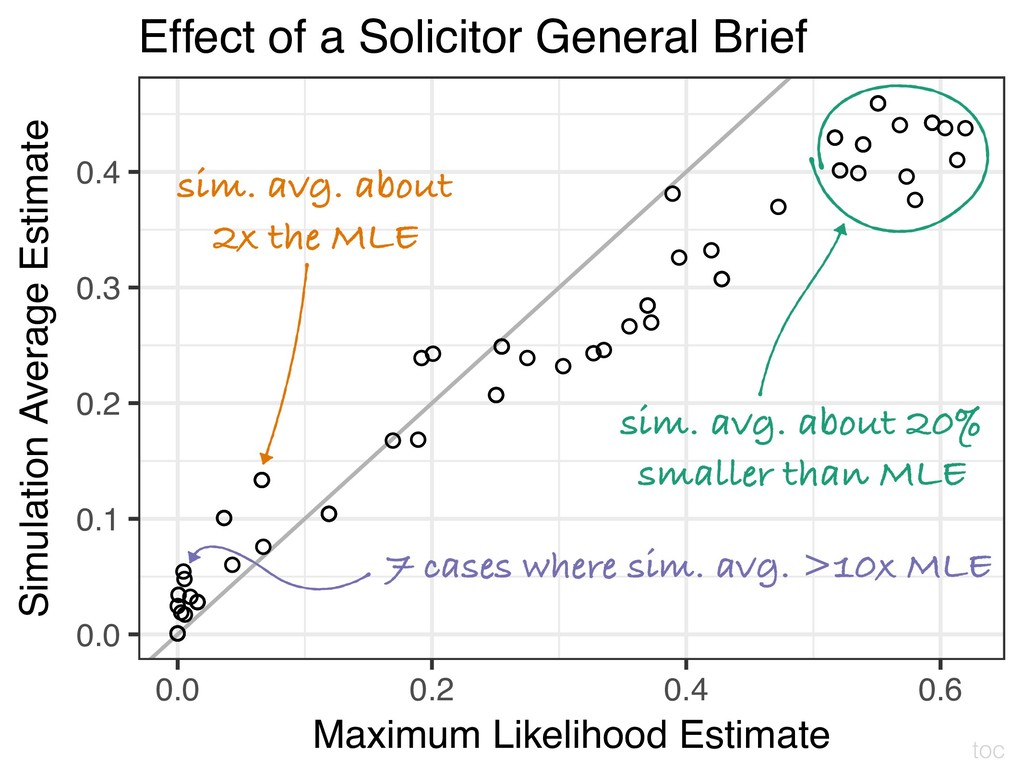
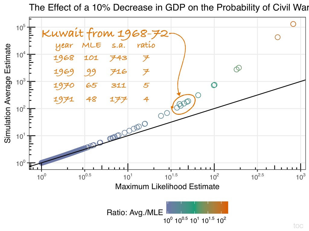
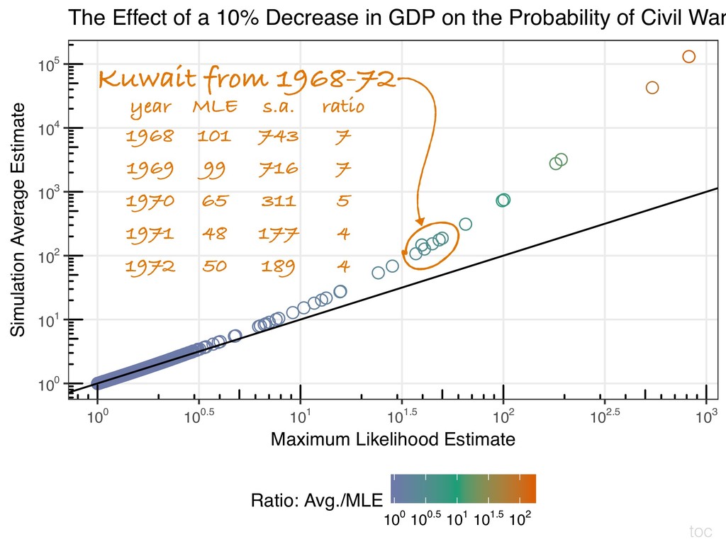
greater than the (upwardly biased) ML estimate. So, of course the average of simulations is more biased than the ML estimate. This additional bias is roughly equal to the transformation-induced bias. 1 2 3
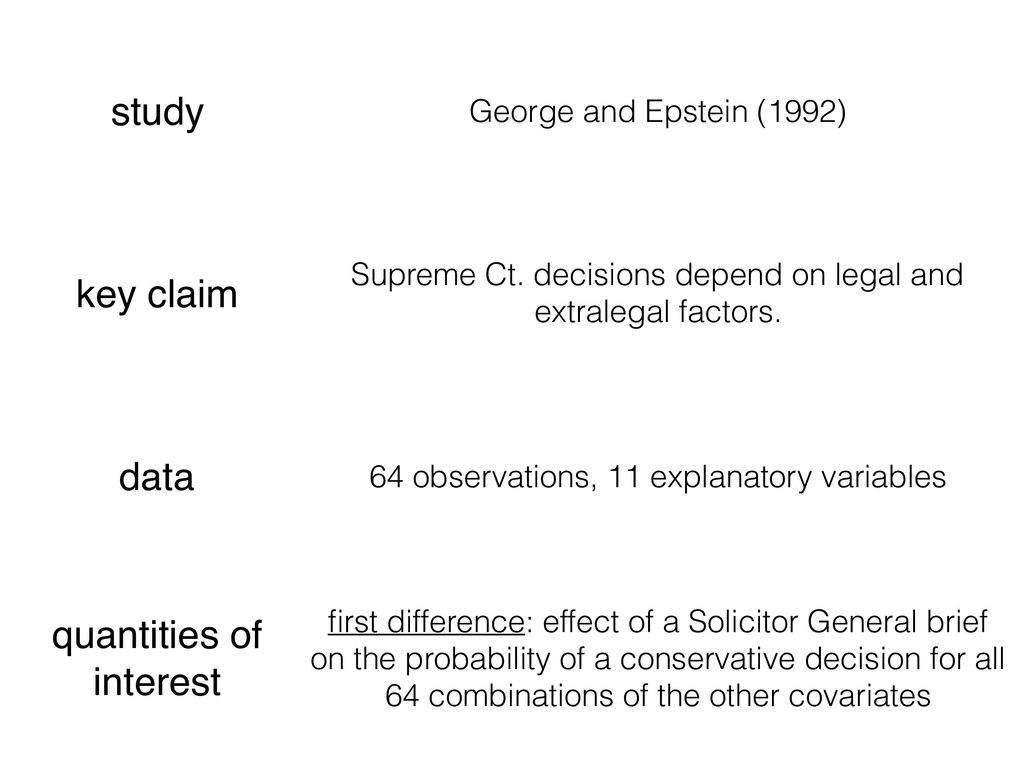
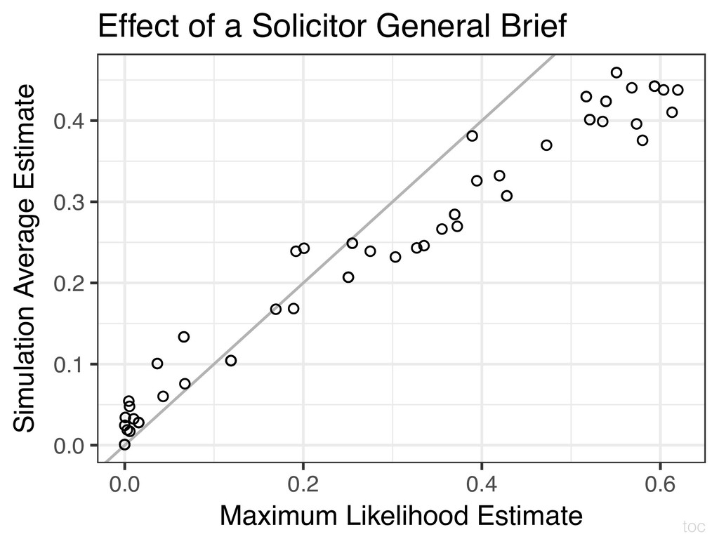
depend on legal and extralegal factors. data 64 observations, 11 explanatory variables quantities of interest first difference: effect of a Solicitor General brief on the probability of a conservative decision for all 64 combinations of the other covariates
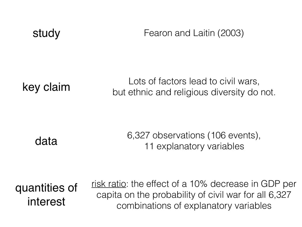
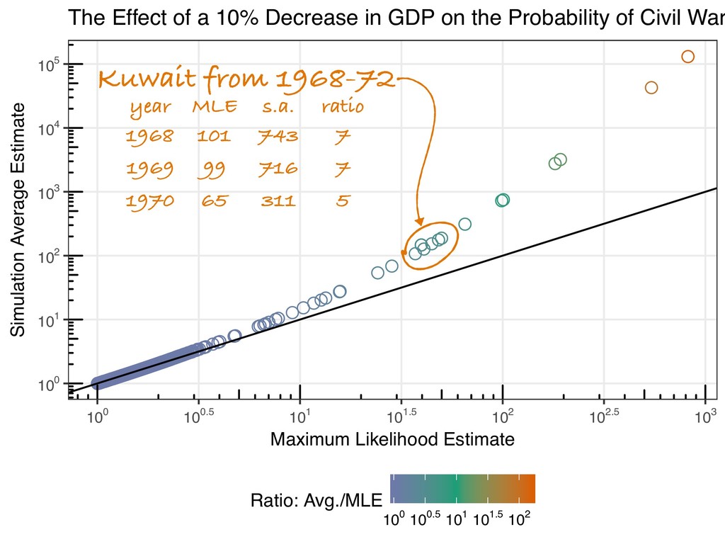
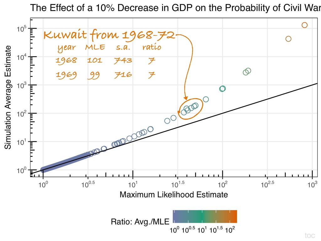
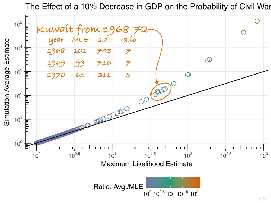
lead to civil wars, but ethnic and religious diversity do not. data 6,327 observations (106 events), 11 explanatory variables quantities of interest risk ratio: the effect of a 10% decrease in GDP per capita on the probability of civil war for all 6,327 combinations of explanatory variables
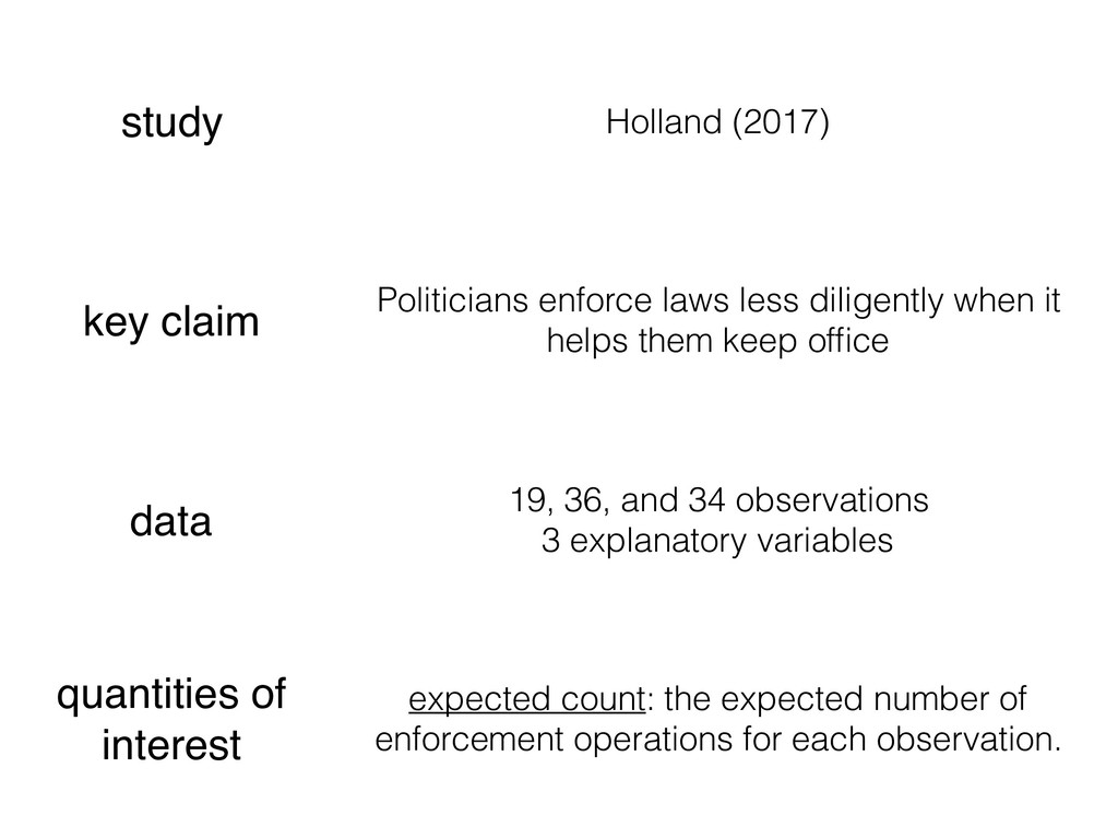
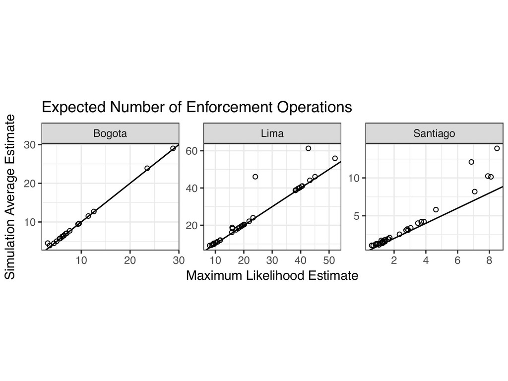
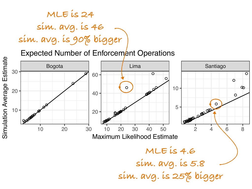
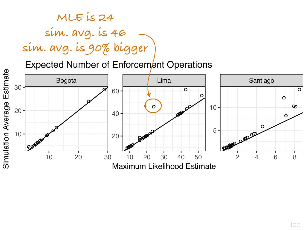
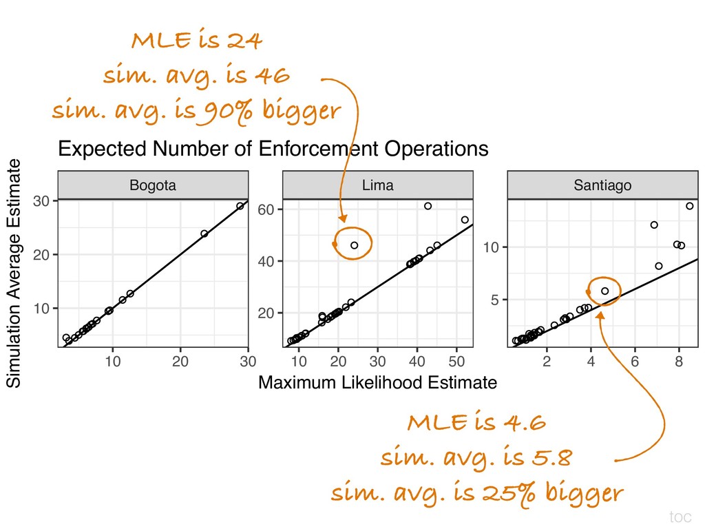
when it helps them keep office data 19, 36, and 34 observations 3 explanatory variables quantities of interest expected count: the expected number of enforcement operations for each observation.
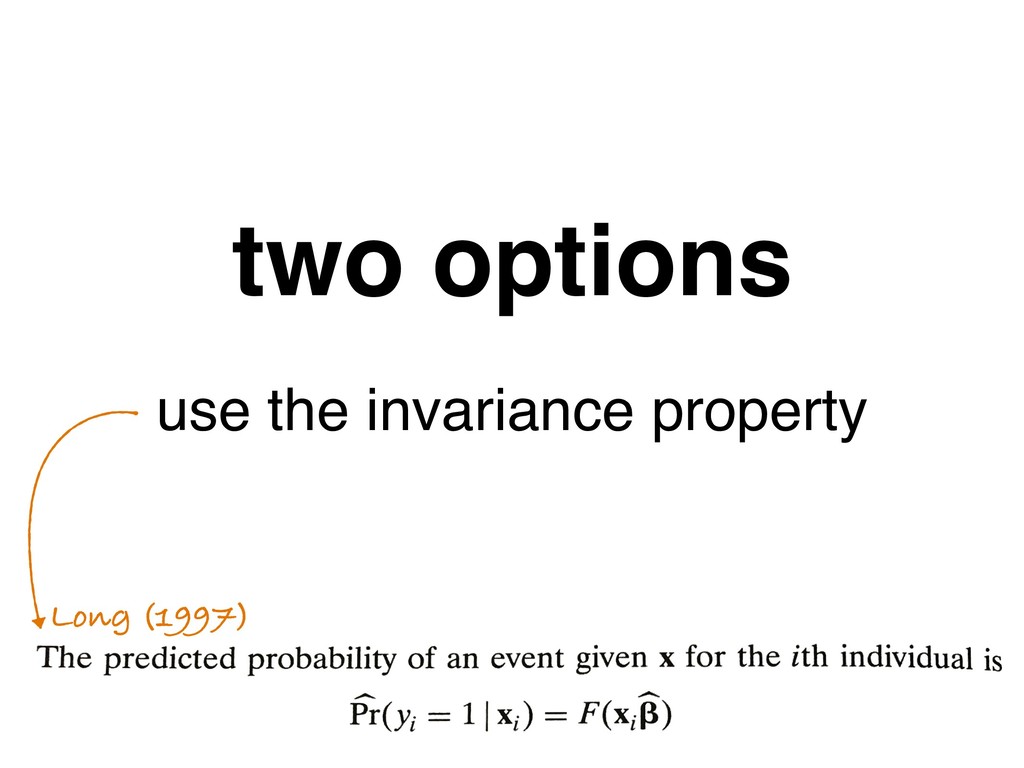
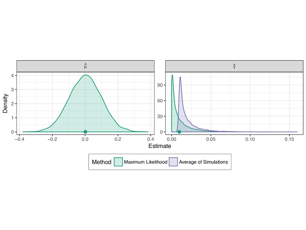
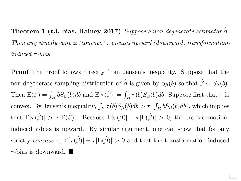
ˆ. Then any strictly convex (concave) ⌧ creates upward (downward) transformation- induced ⌧-bias. Proof The proof follows directly from Jensen’s inequality. Suppose that the non-degenerate sampling distribution of ˆ is given by S (b) so that ˆ ⇠ S (b). Then E(ˆ) = R B bS (b)db and E[⌧(ˆ)] = R B ⌧(b)S (b)db. Suppose first that ⌧ is convex. By Jensen’s inequality, R B ⌧(b)S (b)db > ⌧ ⇥R B bS (b)db ⇤ , which implies that E[⌧(ˆ)] > ⌧[E(ˆ)]. Because E[⌧(ˆ)] ⌧[E(ˆ)] > 0, the transformation- induced ⌧-bias is upward. By similar argument, one can show that for any strictly concave ⌧, E[⌧(ˆ)] ⌧[E(ˆ)] > 0 and that the transformation-induced ⌧-bias is downward. ⌅ toc
any strictly convex (concave) ⌧ guarantees that ˆ ⌧avg. is strictly greater [less] than ˆ ⌧mle. Proof By definition, ˆ ⌧avg. = E h ⌧ ⇣ ˜ ⌘i . Using Jensen’s inequality, we know that E h ⌧ ⇣ ˜ ⌘i > ⌧ h E ⇣ ˜ ⌘i , so that ˆ ⌧avg. > ⌧ h E ⇣ ˜ ⌘i . However, because ˜ ⇠ N h ˆmle, ˆ V ⇣ ˆmle ⌘i , E ⇣ ˜ ⌘ = ˆmle, so that ˆ ⌧avg. > ⌧ ⇣ ˆmle ⌘ . Of course, ˆ ⌧mle = ⌧ ⇣ ˆmle ⌘ by definition, so that ˆ ⌧avg. > ˆ ⌧mle. The proof for concave ⌧ follows similarly. ⌅
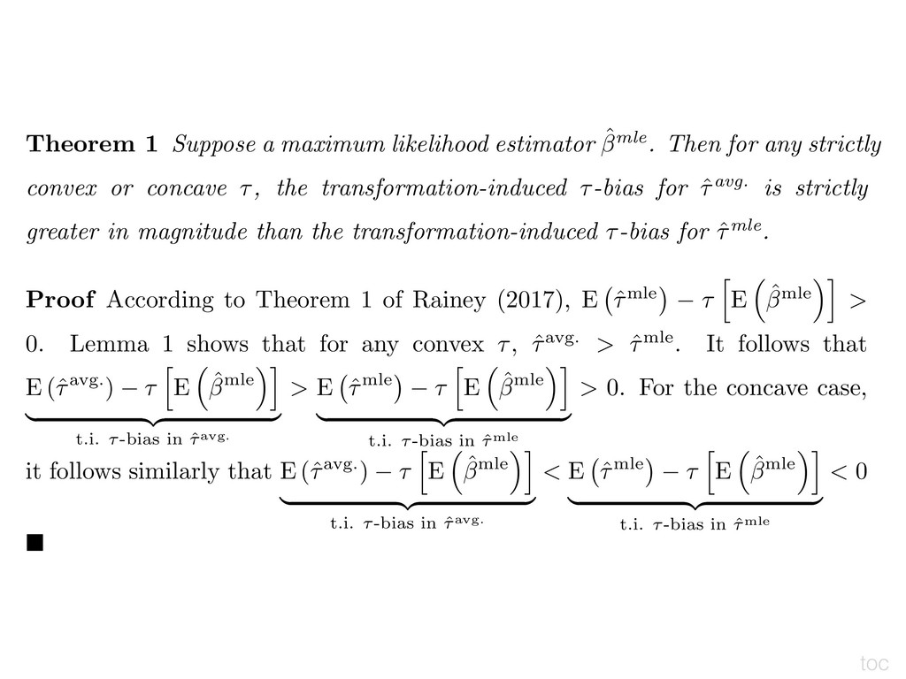
any strictly convex or concave ⌧, the transformation-induced ⌧-bias for ˆ ⌧avg. is strictly greater in magnitude than the transformation-induced ⌧-bias for ˆ ⌧mle. Proof According to Theorem 1 of Rainey (2017), E ˆ ⌧mle ⌧ h E ⇣ ˆmle ⌘i > 0. Lemma 1 shows that for any convex ⌧, ˆ ⌧avg. > ˆ ⌧mle. It follows that E (ˆ ⌧avg.) ⌧ h E ⇣ ˆmle ⌘i | {z } t.i. ⌧-bias in ˆ ⌧avg. > E ˆ ⌧mle ⌧ h E ⇣ ˆmle ⌘i | {z } t.i. ⌧-bias in ˆ ⌧mle > 0. For the concave case, it follows similarly that E (ˆ ⌧avg.) ⌧ h E ⇣ ˆmle ⌘i | {z } t.i. ⌧-bias in ˆ ⌧avg. < E ˆ ⌧mle ⌧ h E ⇣ ˆmle ⌘i | {z } t.i. ⌧-bias in ˆ ⌧mle < 0 ⌅ toc
![Jensen’s inequality: E[g(X)] > g(E[X]) for convex g. e.g., small-sample](https://files.speakerdeck.com/presentations/a5d31e94c89245eb902065fea1f0fe83/slide_44.jpg)