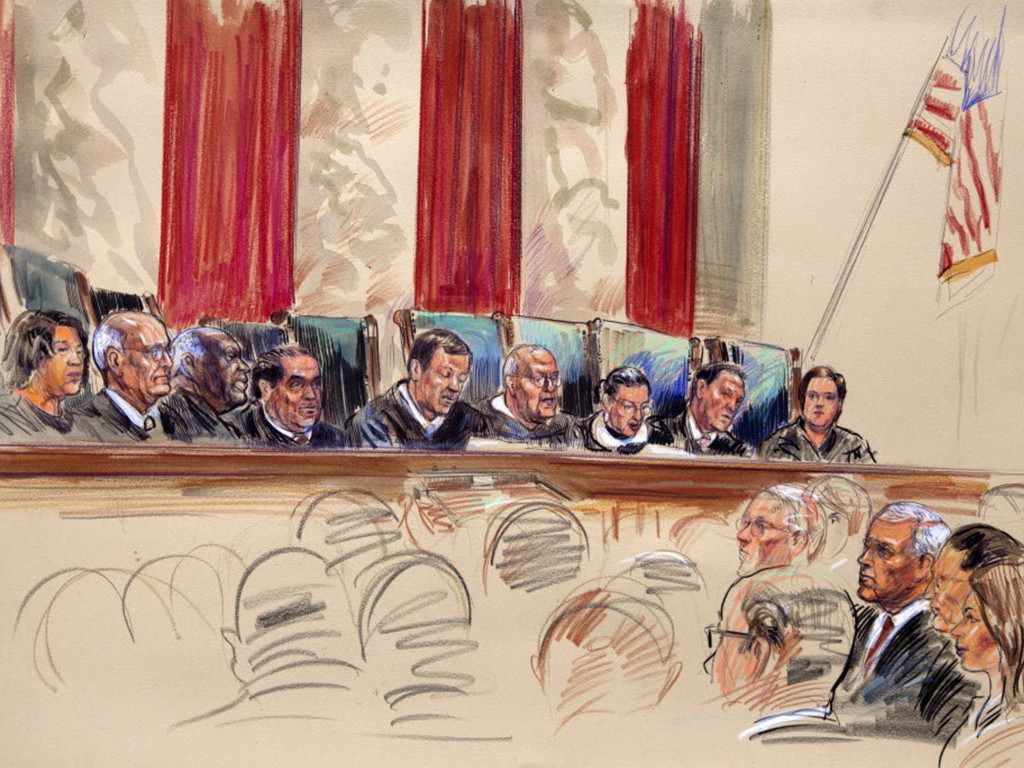
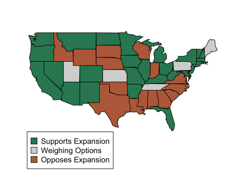
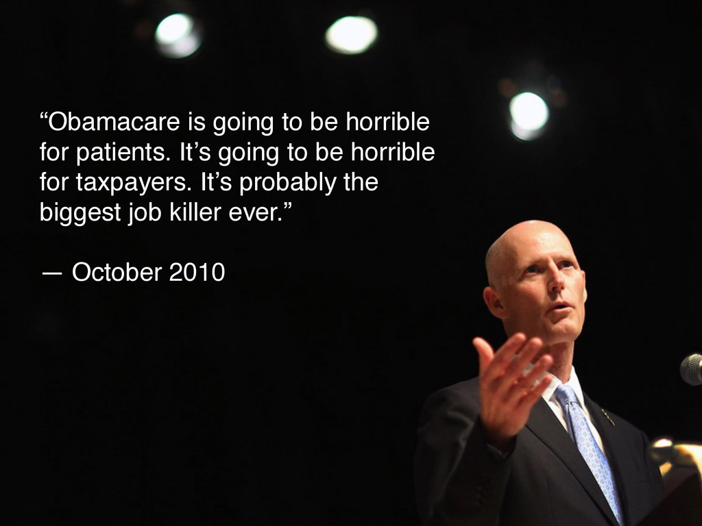
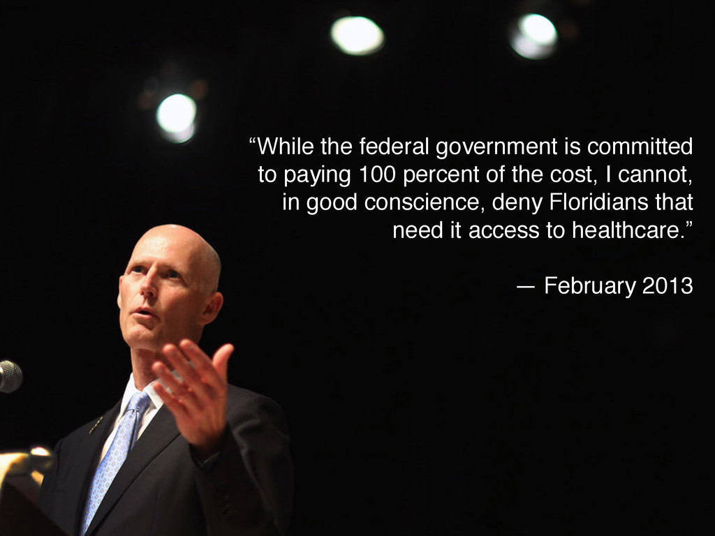
to be horrible for taxpayers. It’s probably the biggest job killer ever.” — October 2010 “While the federal government is committed to paying 100 percent of the cost, I cannot, in good conscience, deny Floridians that need it access to healthcare.” — February 2013
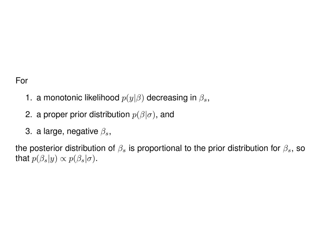
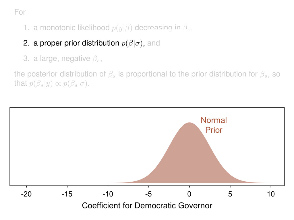
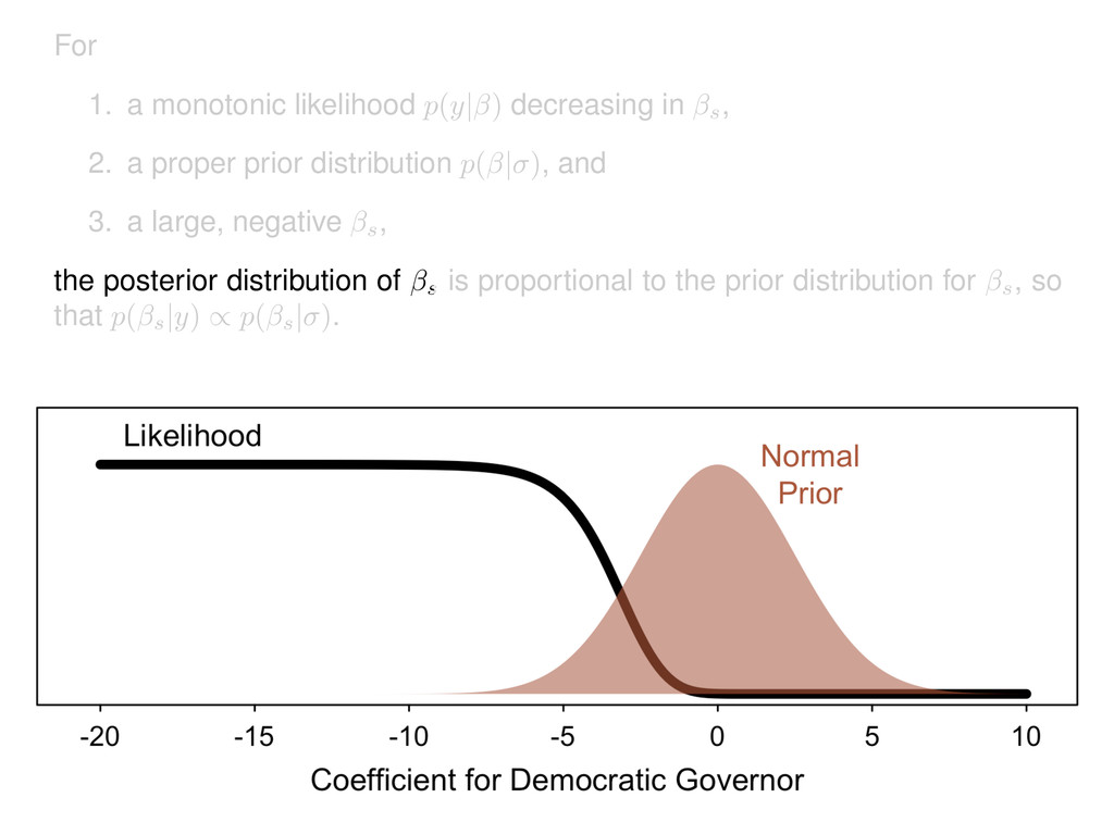
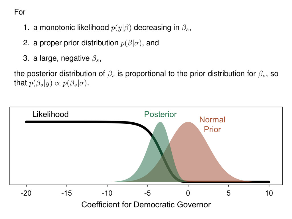
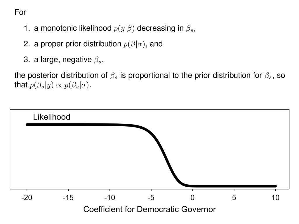
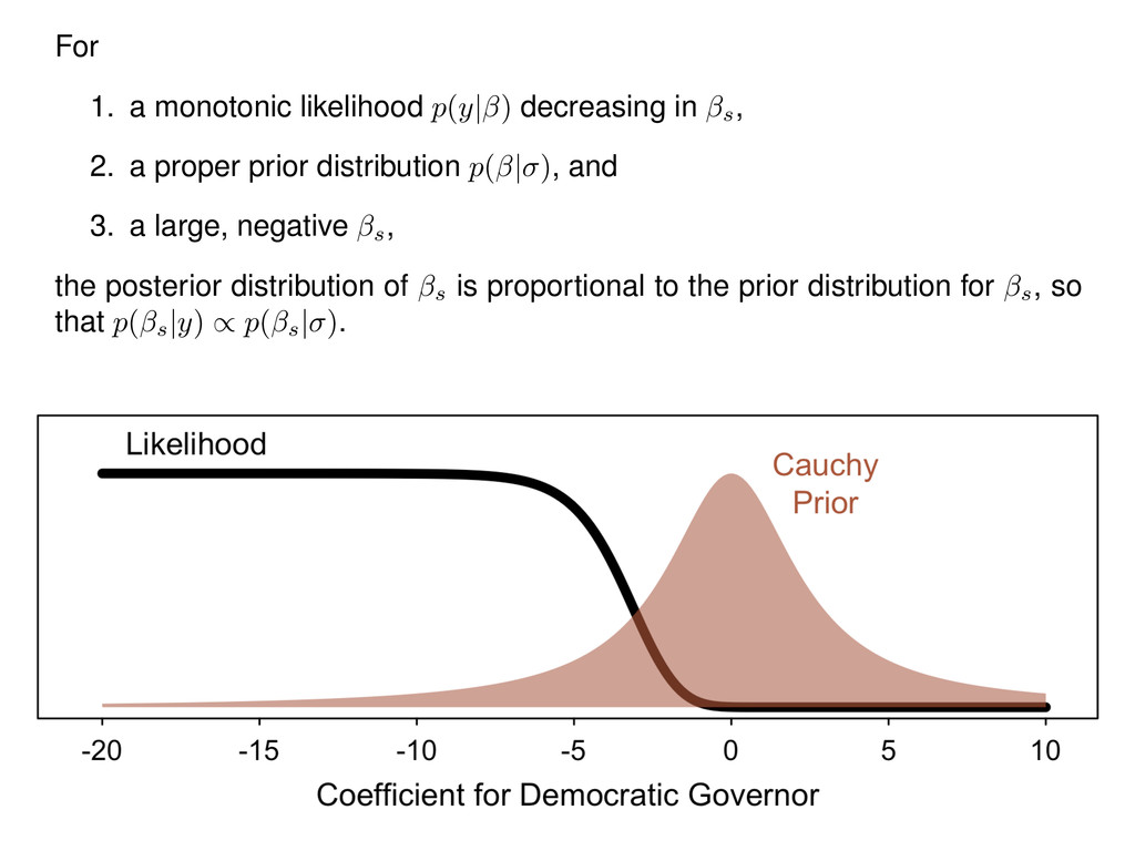
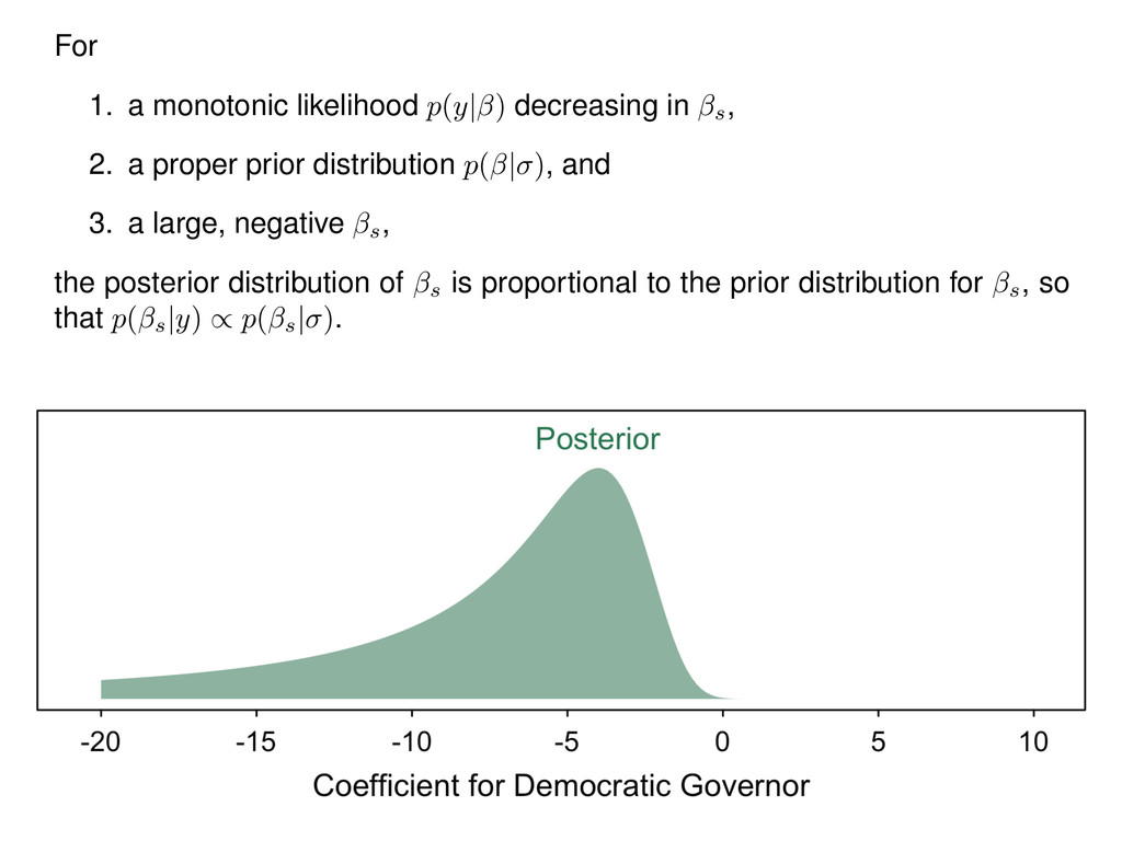
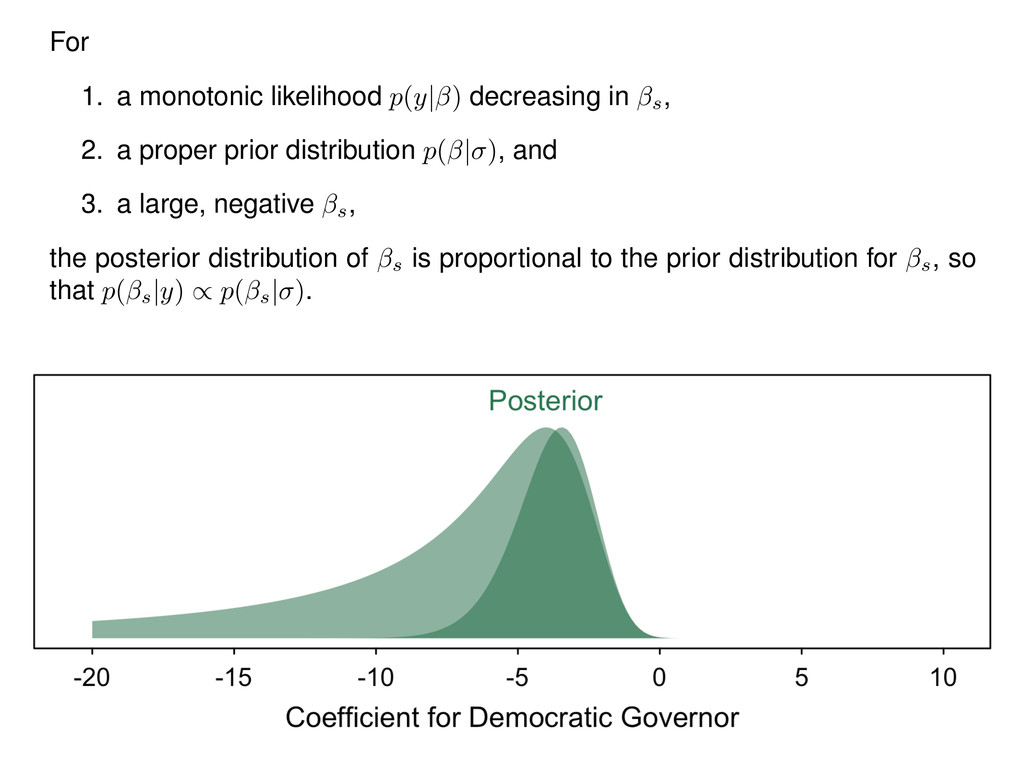
2. a proper prior distribution p( | ) , and 3. a large, negative s, the posterior distribution of s is proportional to the prior distribution for s, so that p( s |y) / p( s | ) .
2. a proper prior distribution p( | ) , and 3. a large, negative s, the posterior distribution of s is proportional to the prior distribution for s, so that p( s |y) / p( s | ) .
2. a proper prior distribution p( | ) , and 3. a large, negative s, the posterior distribution of s is proportional to the prior distribution for s, so that p( s |y) / p( s | ) .
2. a proper prior distribution p( | ) , and 3. a large, negative s, the posterior distribution of s is proportional to the prior distribution for s, so that p( s |y) / p( s | ) .
2. a proper prior distribution p( | ) , and 3. a large, negative s, the posterior distribution of s is proportional to the prior distribution for s, so that p( s |y) / p( s | ) .
2. a proper prior distribution p( | ) , and 3. a large, negative s, the posterior distribution of s is proportional to the prior distribution for s, so that p( s |y) / p( s | ) .
2. a proper prior distribution p( | ) , and 3. a large, negative s, the posterior distribution of s is proportional to the prior distribution for s, so that p( s |y) / p( s | ) .
2. a proper prior distribution p( | ) , and 3. a large, negative s, the posterior distribution of s is proportional to the prior distribution for s, so that p( s |y) / p( s | ) .
2. a proper prior distribution p( | ) , and 3. a large, negative s, the posterior distribution of s is proportional to the prior distribution for s, so that p( s |y) / p( s | ) .
2. a proper prior distribution p( | ) , and 3. a large, negative s, the posterior distribution of s is proportional to the prior distribution for s, so that p( s |y) / p( s | ) .
2. a proper prior distribution p( | ) , and 3. a large, negative s, the posterior distribution of s is proportional to the prior distribution for s, so that p( s |y) / p( s | ) .
2. a proper prior distribution p( | ) , and 3. a large, negative s, the posterior distribution of s is proportional to the prior distribution for s, so that p( s |y) / p( s | ) .
2. a proper prior distribution p( | ) , and 3. a large, negative s, the posterior distribution of s is proportional to the prior distribution for s, so that p( s |y) / p( s | ) .
2. a proper prior distribution p( | ) , and 3. a large, negative s, the posterior distribution of s is proportional to the prior distribution for s, so that p( s |y) / p( s | ) .
2. a proper prior distribution p( | ) , and 3. a large, negative s, the posterior distribution of s is proportional to the prior distribution for s, so that p( s |y) / p( s | ) .
2. a proper prior distribution p( | ) , and 3. a large, negative s, the posterior distribution of s is proportional to the prior distribution for s, so that p( s |y) / p( s | ) .
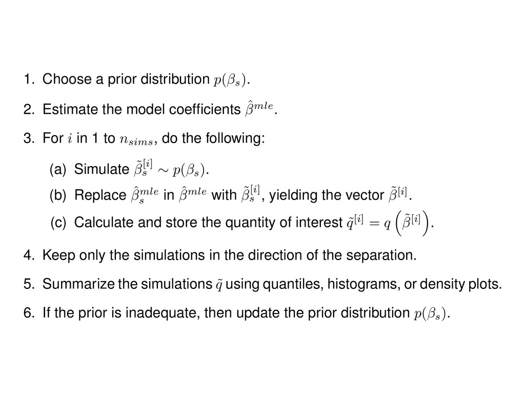
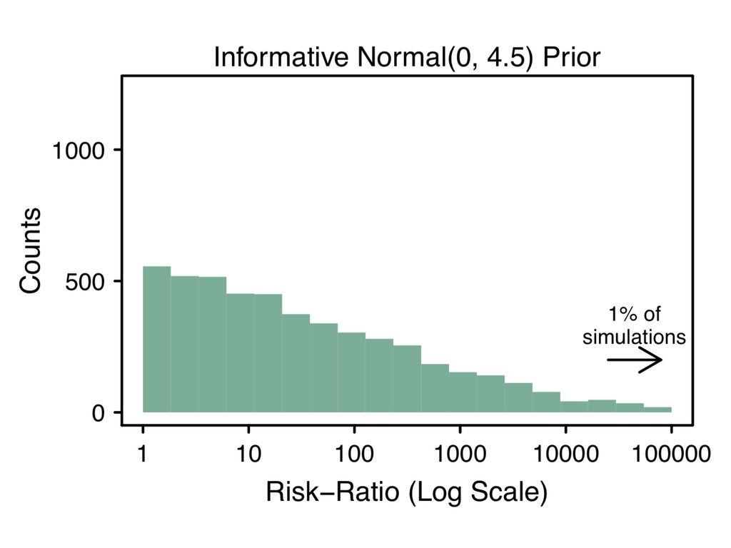
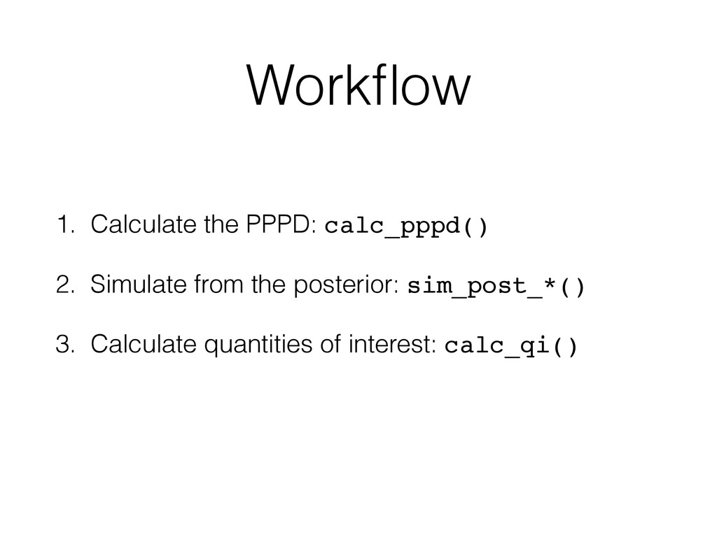
the model coefficients ˆmle . 3. For i in 1 to nsims, do the following: (a) Simulate ˜[i] s ⇠ p( s) . (b) Replace ˆmle s in ˆmle with ˜[i] s , yielding the vector ˜[i] . (c) Calculate and store the quantity of interest ˜ q[i] = q ⇣ ˜[i] ⌘ . 4. Keep only the simulations in the direction of the separation. 5. Summarize the simulations ˜ q using quantiles, histograms, or density plots. 6. If the prior is inadequate, then update the prior distribution p( s) .
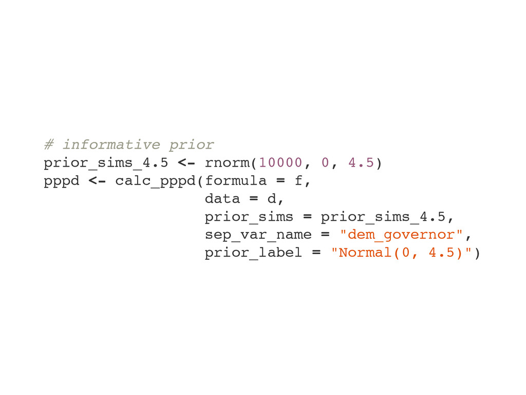
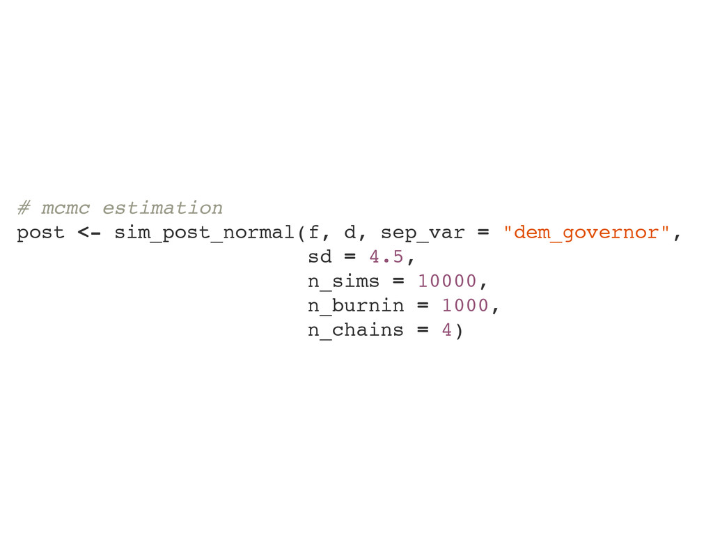
# for rescale() # load and recode data data(politics_and_need) d <- politics_and_need d$dem_governor <- 1 - d$gop_governor d$st_percent_uninsured <- rescale(d$percent_uninsured) # formula to use throughout f <- oppose_expansion ~ dem_governor + percent_favorable_aca + gop_leg + st_percent_uninsured + bal2012 + multiplier + percent_nonwhite + percent_metro
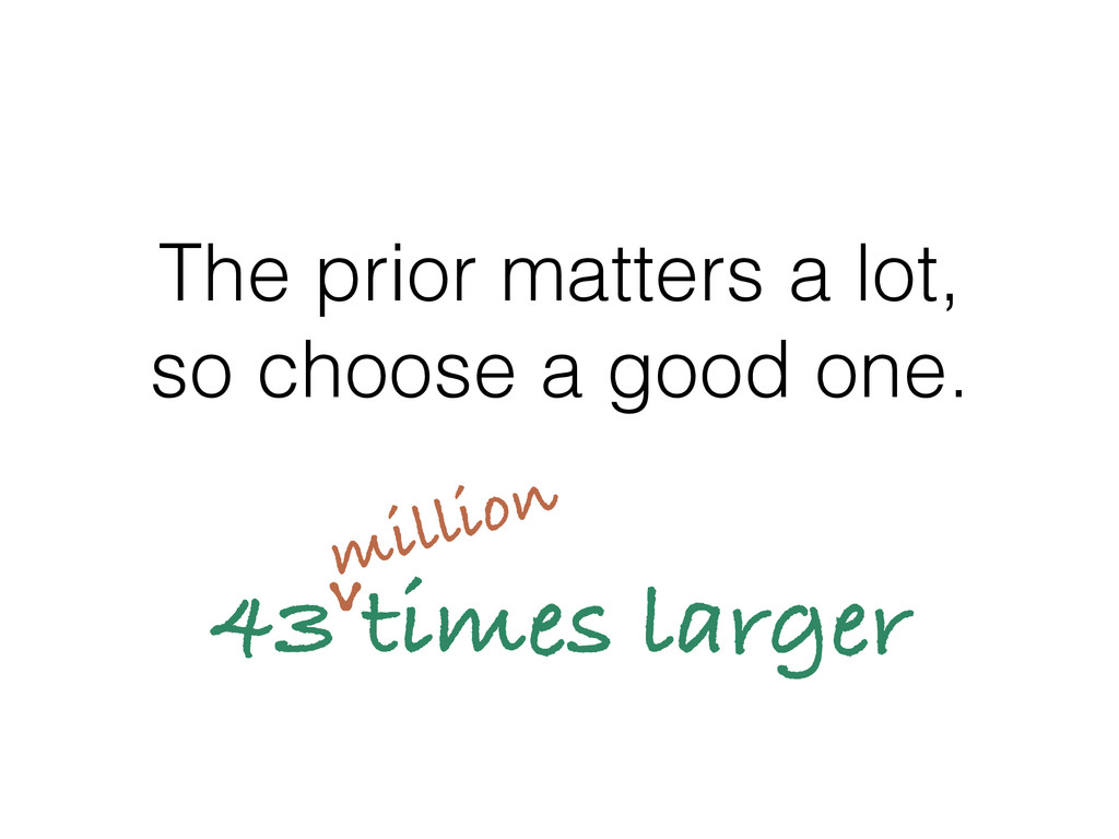
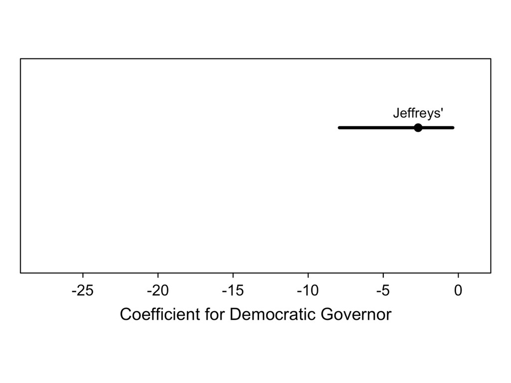
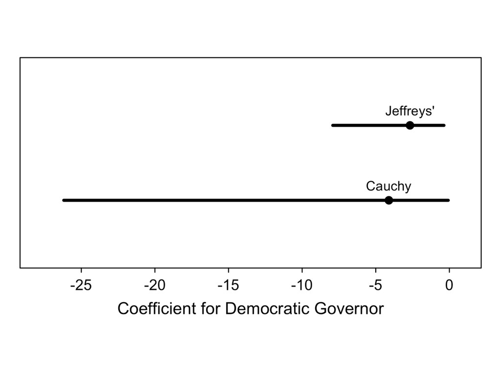
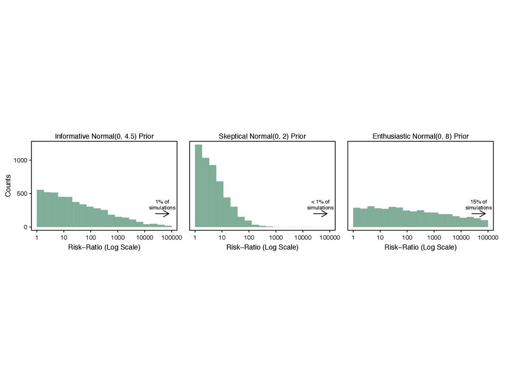
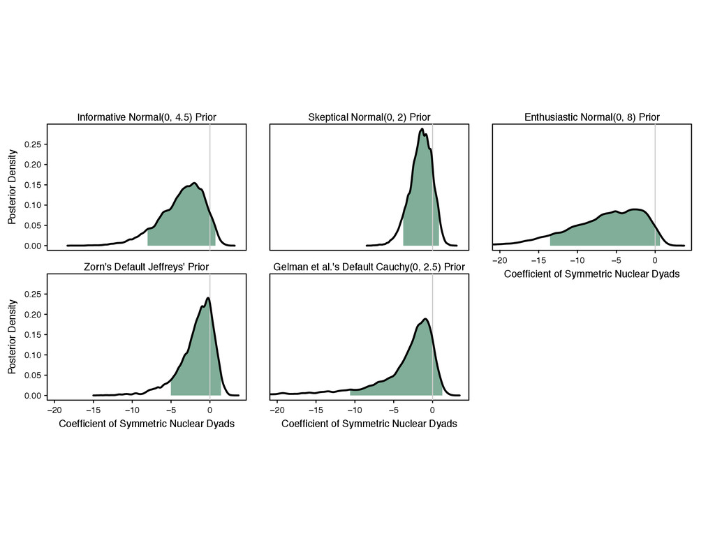
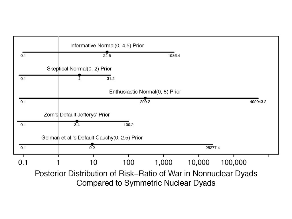
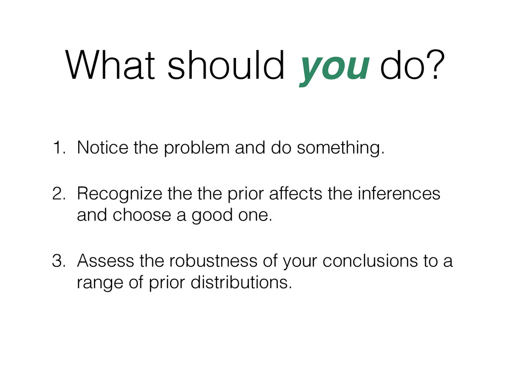
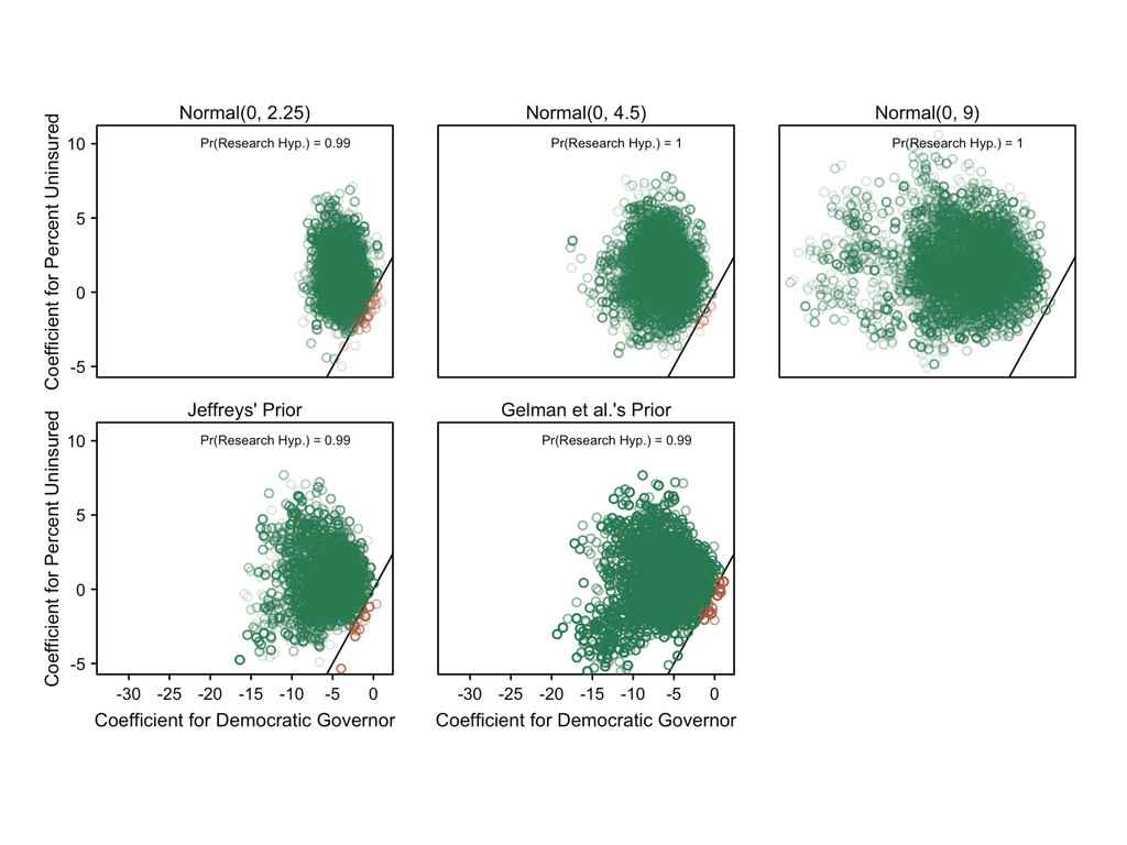
something. 2. Recognize the the prior affects the inferences and choose a good one. 3. Assess the robustness of your conclusions to a range of prior distributions.
2. a proper prior distribution p( | ) , and 3. a large, negative s, the posterior distribution of s is proportional to the prior distribution for s, so that p( s |y) / p( s | ) .
in s, proper prior distribution p( | ) , and large positive [negative] s, the posterior distribution of s is proportional to the prior distribution for s, so that p( s |y) / p( s | ) .
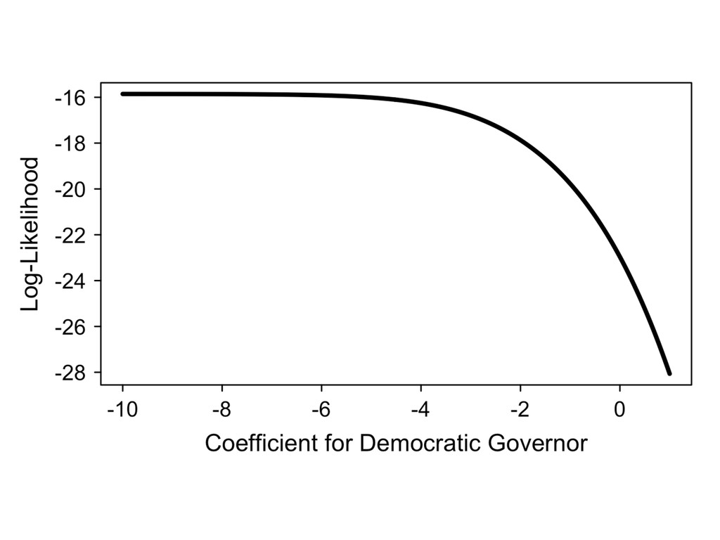
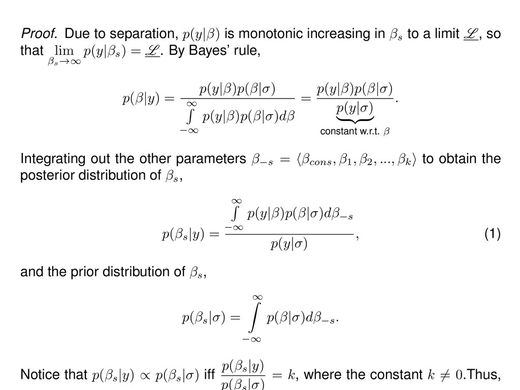
s to a limit L , so that lim s !1 p(y| s ) = L . By Bayes’ rule, p( |y) = p(y| )p( | ) 1 R 1 p(y| )p( | )d = p(y| )p( | ) p(y| ) | {z } constant w.r.t. . Integrating out the other parameters s = h cons , 1, 2, ..., k i to obtain the posterior distribution of s, p( s |y) = 1 R 1 p(y| )p( | )d s p(y| ) , (1) and the prior distribution of s, p( s | ) = 1 Z 1 p( | )d s . Notice that p( s |y) / p( s | ) iff p( s |y) p( | ) = k , where the constant k 6= 0 .Thus,
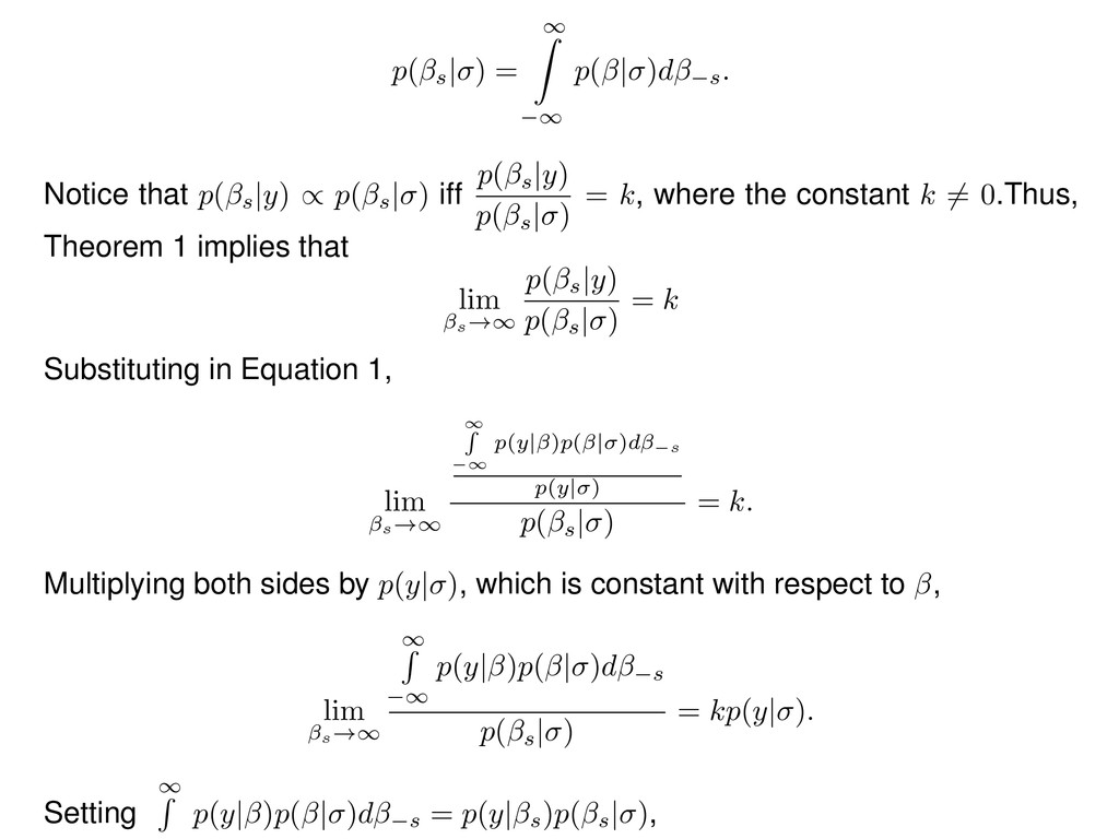
)d s . Notice that p( s |y) / p( s | ) iff p( s |y) p( s | ) = k , where the constant k 6= 0 .Thus, Theorem 1 implies that lim s !1 p( s |y) p( s | ) = k Substituting in Equation 1, lim s !1 1 R 1 p ( y | ) p ( | ) d s p ( y | ) p( s | ) = k. Multiplying both sides by p(y| ) , which is constant with respect to , lim s !1 1 R 1 p(y| )p( | )d s p( s | ) = kp(y| ). Setting 1 R p(y| )p( | )d s = p(y| s )p( s | ) ,
lim s !1 1 R 1 p ( y | ) p ( | ) d s p ( y | ) p( s | ) = k. Multiplying both sides by p(y| ) , which is constant with respect to , lim s !1 1 R 1 p(y| )p( | )d s p( s | ) = kp(y| ). Setting 1 R 1 p(y| )p( | )d s = p(y| s )p( s | ) , lim s !1 p(y| s )p( s | ) p( s | ) = kp(y| ). Canceling p( s | ) in the numerator and denominator, lim s !1 p(y| s ) = kp(y| ).
![Variable Coefficient Confidence Interval Democratic Governor -20.35 [-6,340.06; 6,299.36] %](https://files.speakerdeck.com/presentations/2c081d3823234685a8b857930c592528/slide_18.jpg)
![Variable Coefficient Confidence Interval Democratic Governor -26.35 [-126,979.03; 126,926.33] %](https://files.speakerdeck.com/presentations/2c081d3823234685a8b857930c592528/slide_21.jpg)
![Variable Coefficient Confidence Interval Democratic Governor -26.35 [-126,979.03; 126,926.33] %](https://files.speakerdeck.com/presentations/2c081d3823234685a8b857930c592528/slide_22.jpg)
![Theorem 1. For a monotonic likelihood p(y| ) increasing [decreasing]](https://files.speakerdeck.com/presentations/2c081d3823234685a8b857930c592528/slide_102.jpg)