When BLUE is Not Best

Talk given on March 26, 2015, at "Innovations in Comparative Political Methodology" at Texas A&M University.

Transcript

1. When BLUE Is Not Best
   Non-Normal Errors and the Linear Model
   Carlisle Rainey
   Assistant Professor
   University at Buffalo, SUNY
   Daniel K. Baissa
   Graduate Student
   University at Buffalo, SUNY
   Paper, code, and data at
   carlislerainey.com/research
   

   View Slide

2. Key Point
   Gauss-Markov theorem is an elegant result,
   but it’s not useful for applied researchers.
   

   View Slide

3. Key Point
   Normality matters.
   

   View Slide

4. Background
   

   View Slide

5. yi = Xi + ✏i
   

   View Slide

6. Technical assumptions:
   1. The design matrix is full rank.
   2. The model is correct.
   

   View Slide

7. Additional assumptions:
   1. Errors have mean zero.
   2. Errors have constant, finite variance.
   3. Errors are independent.
   4. Errors follow a normal distribution.
   

   View Slide

8. Additional assumptions:
   1. Errors have mean zero.
   2. Errors have constant, finite variance.
   3. Errors are independent.
   4. Errors follow a normal distribution.
   A1 → consistency
   

   View Slide

9. Additional assumptions:
   1. Errors have mean zero.
   2. Errors have constant, finite variance.
   3. Errors are independent.
   4. Errors follow a normal distribution.
   A1-A4 → BUE
   

   View Slide

10. But is there something
    in between?
    

    View Slide

11. Additional assumptions:
    1. Errors have mean zero.
    2. Errors have constant, finite variance.
    3. Errors are independent.
    4. Errors follow a normal distribution.
    A1-A3 → BLUE
    (Gauss-Markov Theorem)
    

    View Slide

12. But this is not a powerful result.
    

    View Slide

13. Linearity in BLUE
    

    View Slide

14. Linearity in BLUE
    linear model
    or
    linear in the parameters
    

    View Slide

15. Linearity in BLUE
    linear model
    or
    linear in the parameters
    

    View Slide

16. Linearity in BLUE
    linear estimator
    or
    ˆ = 1yy + 2y2 + ... + nyn
    ˆ = My
    

    View Slide

17. Linearity in BLUE
    linearity ≅ easy
    ˆ = My = (X0X) 1X0y
    

    View Slide

18. Linearity in BLUE
    Question:
    BLUE ≅ BUE?
    How large of a deviation from normal errors
    before LS is not approximately BUE?
    

    View Slide

19. −4 −2 0 2 4
    ε
    i
    0.0
    0.1
    0.2
    0.3
    0.4
    Density
    

    View Slide

20. −4 −2 0 2 4
    ε
    i
    0.0
    0.1
    0.2
    0.3
    0.4
    Density
    

    View Slide

21. Restriction to linear estimators
    makes statistical sense only when
    errors are normal.
    

    View Slide

22. Practical Importance
    

    View Slide

23. –Berry (1993)
    “[Even without normally distributed errors]
    OLS coefficient estimators remain
    unbiased and efficient.”
    

    View Slide

24. –Wooldridge (2013)
    “[The Gauss-Markov theorem] justifies the
    use of the OLS method rather than using
    a variety of competing estimators.”
    

    View Slide

25. –Gujarati (2004)
    “We need not look for another linear
    unbiased estimator, for we will not find
    such an estimator whose variance is
    smaller than the OLS estimator.”
    

    View Slide

26. –Berry and Feldman (1993)
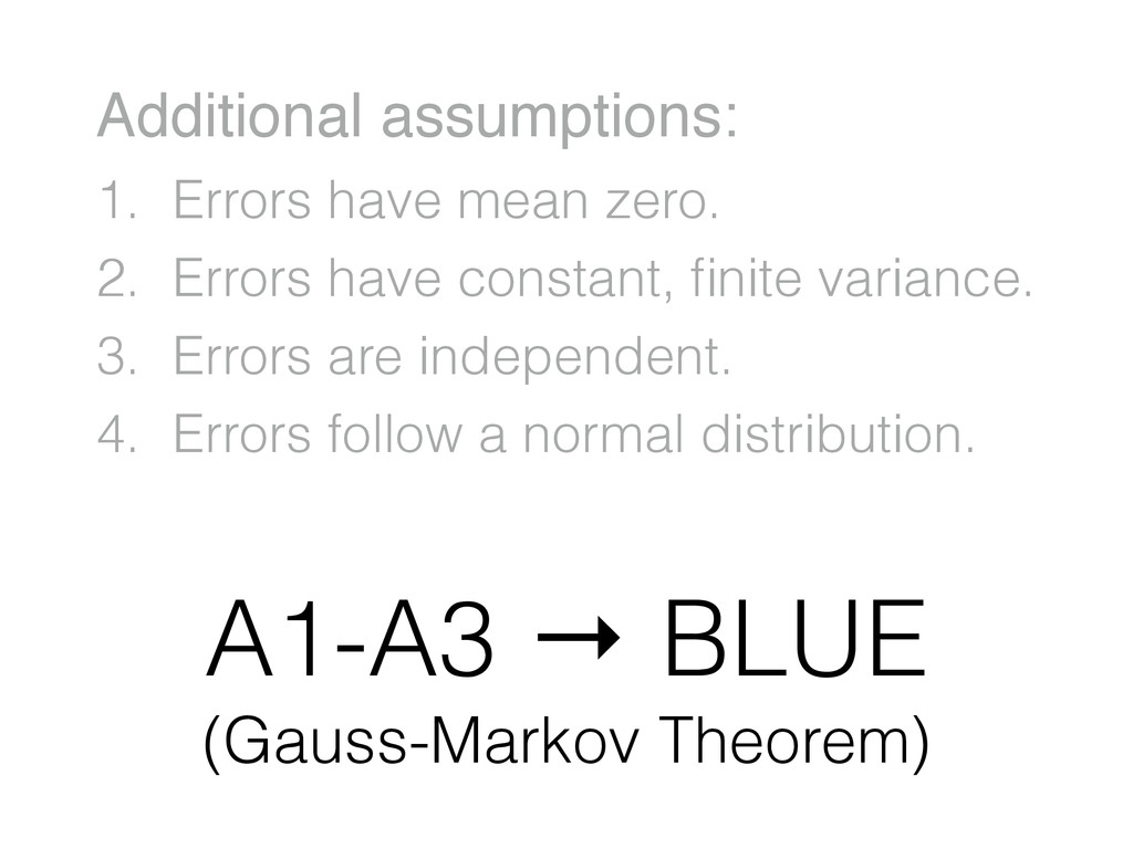
    “An important result in multiple regression is
    the Gauss-Markov theorem, which proves
    that when the assumptions are met, the
    least squares estimators of regression
    parameters are unbiased and efficient.”
    

    View Slide

27. –Berry and Feldman (1993)
    “The Gauss-Markov theorem allows us to
    have considerable confidence in the least
    squares estimators.”
    

    View Slide

28. Gauss-Markov has
    convinced researchers that
    residuals are not important.
    

    View Slide

29. Alternatives
    

    View Slide

30. Skewness
    

    View Slide

31. Heavy Tails
    

    View Slide

32. ˆLS = arg min
    b
    n
    X
    i=1
    (yi Xib)2
    

    View Slide

33. ˆ⇢ = arg min
    b
    n
    X
    i=1
    ⇢(yi Xib)
    

    View Slide

34. Choose function ρ such that the estimator:
    1. performs nearly as well as LS for normal errors
    2. performs much better than LS for non-normal errors.
    

    View Slide

35. −5 0 5
    ε
    i
    0
    20
    40
    60
    ρ(ε
    i
    )
    Square
    

    View Slide

36. −5 0 5
    ε
    i
    0
    2
    4
    6
    8
    ρ(ε
    i
    )
    Absolute Value
    

    View Slide

37. −5 0 5
    ε
    i
    0
    1
    2
    3
    ρ(ε
    i
    )
    Biweight
    

    View Slide

38. Robust estimators are often
    more efficient than LS.
    

    View Slide

39. Robust estimators allow
    unusual cases to be unusual.
    

    View Slide

40. Clark and Golder
    

    View Slide

41. −2 0 2 4 6
    Standardized Residuals
    0
    50
    100
    150
    Counts
    Shapiro−Wilk p−value: 2.8 × 10−18
    

    View Slide

42. −4 −2 0 2 4
    Normal (Theoretical) Quantiles
    0
    5
    10
    Data Quantiles
    ●
    ●
    ●
    ●
    ●
    ●
    ●
    ●
    ●
    ●
    ●
    ●
    ●
    ●
    ●
    ●
    ●
    ●
    ●
    ●
    ●
    ● ●
    ●
    ● ●
    ●
    ●
    ●
    ●
    ●
    ●
    ●● ●
    ●
    ●
    ● ●
    ●
    ●
    ●
    ●
    ●
    ●
    ●●
    ●
    ●
    ●
    ●
    ●
    ●
    ●
    ●
    ●
    ●
    ●
    ●
    ●
    ●
    ●
    ●
    ●
    ●
    ●
    ● ●
    ●
    ●
    ●●
    ●
    ●
    ● ●
    ●
    ●
    ●
    ●
    ●
    ●
    ●
    ●
    ●
    ●
    ●
    ●
    ●
    ●
    ●
    ●
    ●
    ●
    ●
    ●
    ●
    ●
    ●
    ●●
    ●
    ●
    ●
    ●● ●
    ●
    ●
    ●
    ●
    ● ●
    ●
    ●
    ●
    ●
    ●
    ●
    ●
    ●
    ●
    ●
    ●
    ●
    ●
    ●
    ●
    ●
    ●
    ●
    ●
    ●
    ●
    ●
    ●
    ●
    ●
    ●
    ●
    ●
    ●
    ●
    ●
    ●
    ●
    ●
    ● ●
    ●
    ●
    ●
    ●
    ● ●
    ● ●
    ● ● ●
    ●
    ●
    ●
    ●
    ●
    ● ●
    ●
    ●
    ●
    ●
    ●
    ●
    ●
    ●
    ●
    ●
    ●
    ●
    ●
    ●
    ●
    ●
    ●
    ●
    ●
    ●
    ●
    ●
    ●
    ● ●
    ●
    ●
    ●
    ●
    ●
    ●
    ●
    ●
    ●
    ●
    ●
    ●
    ●
    ●
    ●
    ●
    ●
    ●
    ●
    ●
    ●
    ●
    ●
    ●
    ●
    ●
    ●
    ●
    ●
    ●
    ●
    ●
    ●
    ●
    ●
    ●
    ●
    ●
    ●
    ●
    ●
    ●
    ● ●
    ●
    ●
    ●
    ●
    ●
    ●
    ●
    ●
    ●
    ●
    ●
    ●
    ●
    ●
    ●
    ●
    ●
    ●
    ●
    ●
    ●
    ●
    ● ●
    ●
    ●
    ●
    ●
    ●
    ● ● ●
    ● ●
    ●
    ●
    ●
    ●●
    ●
    ●
    ●
    ●
    ●
    ●●
    ●
    ●
    ●
    ● ●
    ●
    ●
    ●
    ●
    ●
    ●
    ●
    ● ●
    ●
    ●
    ●
    ●
    ●
    ●
    ●
    ●
    ● ●
    ●
    ●●
    ●
    ●●
    ●
    ●
    ●
    ●
    ●
    ●
    ●
    ●
    ● ●
    ●
    ●
    ●
    ●
    ●
    ●
    ●
    ●
    ●
    ●
    ●
    ●
    ●
    ●
    ●
    ●●
    ●
    ●
    ●
    ●
    ●
    ●
    ●
    ●
    ●
    ●
    ●
    ●
    ●
    ●
    ●
    ●
    ●
    ●
    ●
    ●
    ●
    ●
    ●
    ●
    ●
    ●
    ●
    ●
    ●
    ●
    ●
    ●
    ●
    ●
    ●
    ●
    ●
    ●
    ●
    ●
    ●
    ●●
    ●
    ● ●
    ●
    ●
    ●
    ●
    ●
    ●
    ●
    ●
    ●
    ●
    ●
    ●
    ●
    ●
    ●
    ●
    ●
    ●
    ●
    ●
    ●
    ●
    ●
    ●
    ●
    ●
    ●
    ●
    ●
    ●●
    ●
    ●
    ●
    ● ●
    ●
    ●
    ●
    ●
    ●
    ●
    ●
    ●
    ●
    ●
    ●
    ●
    ●
    ●
    ●
    ●
    ●
    ● ●
    ●
    ●
    ●
    ●
    ●
    ●
    ● ● ●
    ●
    ●
    ●
    ●
    ●
    ●
    ●
    ●
    ●
    ●
    ●
    ●
    ●
    ●
    ●
    ●
    ●
    ●
    ●
    ●
    ●
    ●
    ●
    ●
    ●
    ●
    ●
    ●
    ●
    ●
    ●
    ●
    ●
    ●
    ●
    ●
    ●
    ●
    Chile (1953)
    Thailand (1988)
    Brazil (1962)
    

    View Slide

43. −4 −2 0 2 4
    Normal (Theoretical) Quantiles
    −1.0
    −0.5
    0.0
    0.5
    1.0
    Data Quantiles
    Log Transformation
    ●
    ●
    ●
    ●
    ●
    ●
    ●
    ●
    ●
    ●
    ●
    ●
    ●
    ●
    ●
    ●
    ●
    ●
    ●
    ●
    ●
    ●
    ●
    ●
    ●
    ●
    ●
    ●
    ●
    ●
    ●
    ●
    ●
    ●
    ●
    ●
    ●
    ●
    ●
    ●
    ●
    ●
    ●
    ●
    ●
    ●
    ●
    ●
    ●
    ●
    ●
    ●
    ●
    ●
    ●
    ●
    ●
    ●
    ●
    ●
    ●
    ●
    ●
    ●
    ●
    ●
    ●
    ●
    ●
    ●
    ●●
    ●
    ●
    ●
    ●
    ●
    ●
    ●
    ●
    ●
    ●
    ●
    ●
    ●
    ●
    ●
    ●
    ●
    ●
    ●
    ●
    ●
    ●
    ●●
    ●
    ●
    ●
    ●
    ●
    ●
    ●
    ●
    ●●
    ●
    ●
    ●
    ●
    ●
    ●●
    ●
    ●
    ●
    ●
    ●
    ●
    ●
    ●
    ●
    ●
    ●
    ●
    ●
    ●
    ●
    ●
    ●
    ●
    ●
    ●
    ●
    ●
    ●
    ●
    ●
    ●
    ●
    ●
    ●
    ●●
    ●●
    ●
    ●
    ●
    ●
    ●
    ● ●
    ●
    ●
    ●
    ● ●
    ●
    ●
    ●
    ●
    ●
    ●
    ●
    ●●
    ●
    ●
    ●
    ●
    ●
    ●
    ●
    ●
    ●
    ●
    ●
    ●
    ●
    ●
    ●
    ●
    ●
    ●
    ●
    ●
    ●
    ●
    ●
    ●
    ●
    ●●
    ●
    ●
    ●
    ●
    ●
    ●
    ●
    ●
    ●
    ●
    ●
    ●
    ●
    ●
    ●
    ●
    ●
    ●
    ●
    ●
    ●
    ●
    ●
    ●
    ●
    ●
    ●
    ●
    ●
    ●
    ●
    ●
    ●
    ●
    ●
    ●
    ●
    ●
    ●
    ●
    ●
    ●
    ●
    ●
    ●
    ●
    ●
    ●
    ●
    ●
    ●
    ●
    ●
    ●
    ●
    ●
    ●
    ●
    ●
    ●
    ●
    ●
    ●
    ●
    ●
    ●
    ●
    ●
    ●
    ●
    ●
    ●
    ●●
    ●
    ●
    ●
    ●
    ●
    ●●
    ●
    ●
    ●
    ●
    ●
    ●
    ●
    ●
    ●
    ●
    ●
    ●
    ●
    ●
    ●
    ●
    ●
    ●
    ●
    ●
    ●
    ●
    ●
    ●
    ●
    ●
    ●
    ●
    ●
    ●
    ●
    ●
    ●
    ●
    ●
    ●●
    ●
    ●
    ●
    ●
    ●
    ●
    ●
    ●
    ●
    ●
    ●
    ●
    ●
    ●
    ●
    ●
    ●
    ●
    ●
    ●
    ●
    ●
    ●
    ●
    ●
    ●
    ●
    ●
    ●
    ●
    ●
    ●
    ●
    ●
    ●
    ●
    ●
    ●
    ●
    ●
    ●
    ●
    ●
    ●
    ●
    ●
    ●
    ●
    ●
    ●
    ●
    ●
    ●
    ●
    ●
    ●
    ●
    ●
    ●
    ●
    ●●
    ●
    ●
    ●
    ●
    ●
    ●
    ●●
    ●
    ●
    ●
    ●
    ●
    ●
    ●
    ●
    ●
    ●
    ●
    ●
    ●
    ●
    ●
    ●
    ●
    ●
    ●
    ●
    ●
    ●
    ●
    ●
    ●
    ●
    ●
    ●
    ●
    ●
    ●
    ●
    ●●
    ●
    ●
    ●
    ●
    ●
    ●
    ●
    ●
    ●
    ●
    ●
    ●
    ●
    ●
    ●
    ●
    ●
    ●
    ●
    ●
    ●
    ●
    ●
    ●
    ●
    ●
    ●
    ●
    ●
    ●
    ●
    ●
    ●
    ●
    ●
    ●
    ●
    ●
    ●
    ●
    ●
    ●
    ●
    ●
    ●
    ●
    ●
    ●
    ●
    ●
    ●
    ●
    ●
    ●
    ●
    ●
    ●
    ●
    ●
    ●
    ●
    ●
    ●
    ●
    ●
    ●
    ●
    ●
    ●
    ●
    ●
    −4 −2 0 2 4
    Normal (Theoretical) Quantiles
    Box−Cox Tranformation with λ = −1 3
    ●
    ●
    ●
    ●
    ●
    ●
    ●
    ●
    ●
    ●
    ●
    ●
    ●
    ●
    ●
    ●
    ●
    ●
    ●
    ●
    ●
    ●
    ●
    ●
    ●
    ●
    ●
    ●
    ●
    ●
    ●
    ●
    ●●
    ●
    ●
    ●
    ●
    ●
    ●
    ●
    ●
    ●
    ●
    ●
    ●
    ●
    ●
    ●
    ●
    ●
    ●
    ●
    ●
    ●
    ●
    ●
    ●
    ●
    ●
    ●
    ●
    ●
    ●
    ●
    ●
    ● ●
    ●
    ●
    ●●
    ●
    ●
    ● ●
    ●
    ●
    ●
    ●
    ●
    ●
    ●
    ●
    ●
    ●
    ●
    ●
    ●
    ●
    ●
    ●
    ●
    ●
    ●
    ●
    ●
    ●
    ●
    ●
    ●
    ●
    ●
    ●
    ● ●
    ●
    ●
    ●
    ●
    ●
    ●
    ●
    ●
    ●●
    ●
    ●
    ●
    ●
    ●
    ●
    ●
    ●
    ●
    ●
    ●
    ●
    ●
    ●
    ●
    ●
    ●
    ●
    ●
    ●
    ●
    ●
    ●
    ●
    ●
    ●
    ●
    ●
    ●●
    ●
    ●
    ●
    ●
    ● ● ●
    ●
    ● ●
    ●
    ●
    ●
    ●
    ●
    ●
    ●
    ●
    ●
    ●●
    ●
    ●
    ●
    ●
    ●
    ●●
    ●
    ●
    ●
    ●
    ●
    ●
    ●
    ●
    ●
    ●
    ●
    ●
    ●
    ●
    ●
    ●
    ● ●
    ●●
    ●
    ●
    ●
    ●
    ●
    ●
    ●
    ●
    ●
    ●
    ●
    ●
    ●
    ●
    ●
    ●●
    ●
    ●
    ●
    ●
    ●
    ●
    ●
    ●
    ●
    ●
    ●
    ●
    ●
    ●
    ●
    ●●
    ●
    ●
    ●
    ●●
    ●
    ● ●
    ●
    ●
    ●
    ●
    ●
    ●
    ●
    ●
    ●
    ●
    ●
    ●
    ●
    ●
    ●
    ●
    ●
    ●
    ●
    ●
    ●
    ●
    ●
    ●
    ●
    ●
    ●
    ●
    ●
    ●
    ●●
    ●
    ●
    ●
    ●
    ●
    ●
    ●
    ●
    ●
    ●
    ●
    ●
    ●
    ●
    ● ●
    ●
    ●●
    ●
    ●
    ●
    ●
    ●
    ●
    ●
    ●
    ●
    ●
    ●
    ●
    ●
    ●
    ●
    ●
    ●
    ●
    ●
    ●
    ● ●
    ●
    ●●
    ●
    ●
    ●
    ●
    ●
    ●
    ●
    ●
    ● ●
    ●
    ●
    ●
    ●
    ●
    ●
    ●
    ● ●
    ●
    ●
    ●
    ●
    ●
    ●
    ●
    ●
    ●
    ●
    ●
    ●
    ●
    ●
    ●
    ●
    ●
    ●
    ●
    ●
    ●
    ●
    ●
    ●
    ●
    ●
    ●
    ●
    ●
    ●
    ●
    ●
    ●
    ●
    ●
    ●
    ●
    ●
    ●
    ●
    ●
    ●
    ●
    ●
    ●
    ●
    ●
    ●
    ●
    ●●
    ●
    ● ●
    ●
    ●
    ●
    ●
    ●
    ●
    ●
    ●
    ●
    ●
    ●
    ●
    ●
    ●
    ●
    ●
    ●
    ●
    ●
    ●
    ●
    ● ●
    ●
    ●
    ●
    ●
    ●
    ●
    ●
    ●
    ●
    ●
    ●
    ●
    ●
    ●
    ●
    ●
    ●
    ●
    ●
    ●
    ●
    ●
    ●
    ●
    ●
    ●
    ●
    ●
    ●
    ●
    ●
    ●
    ●●
    ●
    ●
    ●
    ●
    ●
    ●
    ●
    ●
    ●
    ●
    ●
    ●
    ●
    ●
    ●
    ●
    ●
    ●
    ●
    ●
    ●
    ●
    ●
    ●
    ●
    ●
    ●
    ●
    ●
    ●
    ●
    ●
    ●
    ●
    ●
    ●
    ●
    ●
    ●
    ●
    ●
    ●
    ●
    ●
    ●
    

    View Slide

44. −3 −2 −1 0 1 2 3 4
    Standardized Residuals
    0
    50
    100
    Counts
    Log Transformation
    Shapiro−Wilk p−value: 1.6 × 10−6
    −3 −2 −1 0 1 2 3 4
    Standardized Residuals
    Box−Cox Tranformation with λ = −1 3
    Shapiro−Wilk p−value: 0.002
    

    View Slide

45. 0
    5
    10
    15
    Effect of ENEG
    Least Squares, No Transformation Least Squares, Box−Cox Transformation
    1 2 5 20 50 150
    District Magnitude
    0
    5
    10
    15
    Effect of ENEG
    Biweight, No Transformation
    1 2 5 20 50 150
    District Magnitude
    Biweight, Box−Cox Transformation
    

    View Slide

46. 0
    5
    10
    15
    Effect of ENEG
    Least Squares, No Transformation Least Squares, Box−Cox Transformation
    1 2 5 20 50 150
    District Magnitude
    0
    5
    10
    15
    Effect of ENEG
    Biweight, No Transformation
    1 2 5 20 50 150
    District Magnitude
    Biweight, Box−Cox Transformation
    

    View Slide

47. Substantive Takaways
    

    View Slide

48. Substantive Takaways
    The theory is wrong.
    

    View Slide

49. Substantive Takaways
    The theory is wrong.
    We’ve got lots of evidence in favor of the theory.
    • Theoretical
    • Observational studies
    • Quasi-experiments
    • Lab experiments
    

    View Slide

50. Substantive Takaways
    The theory is wrong.
    The estimates are suggest the effects might be smaller
    or larger than Clark and Golder’s analysis suggests.
    

    View Slide

51. Substantive Takaways
    The theory is wrong.
    

    View Slide

52. Substantive Takaways
    We can learn from the residuals.
    

    View Slide

53. −0.6 −0.4 −0.2 0.0 0.2 0.4 0.6
    Residuals from Least Squares Estimates
    with Box−Cox Transformation
    −0.5
    0.0
    0.5
    Residuals from Biweight Estimates
    with Box−Cox Transformation
    ●
    ●
    ●
    ●
    ●
    ●
    ●
    ●
    ●
    ●
    ●
    ●
    ●
    ●
    ●
    ●
    ●
    ●
    ●
    ●
    ●
    ●
    ●
    ●
    ●
    ●
    ●
    ●
    ●
    ●
    ●
    ●
    ●
    ●
    ●
    ●
    ●
    ●
    ●
    ●
    ●
    ●
    ●
    ●
    ●
    ●
    ●
    ●
    ●
    ●
    ●
    ●
    ●
    ●
    ●
    ●
    ●●
    ●
    ●
    ●
    ●
    ●
    ●
    ●
    ●
    ●
    ●
    ●
    ●
    ●
    ●
    ●
    ●
    ●
    ●
    ●
    ●
    ●
    ●
    ●
    ●
    ●
    ●
    ●
    ●
    ●
    ●
    ●
    ●
    ●
    ●
    ●
    ●
    ●
    ●
    ●
    ●
    ●
    ●
    ●
    ●
    ●
    ●
    ●
    ●
    ●
    ●
    ●
    ●
    ●
    ●●
    ●
    ●
    ●
    ●
    ●
    ●
    ●
    ●
    ●
    ●
    ●
    ●
    ●
    ●
    ●
    ●
    ●
    ●
    ●
    ●
    ●
    ●
    ●
    ●
    ●
    ●
    ●
    ●
    ●
    ● ●
    ●
    ●
    ●●
    ●
    ●
    ●
    ● ●
    ●
    ●
    ●
    ●
    ●
    ●
    ●
    ●
    ●
    ●
    ●
    ●
    ●
    ●
    ●
    ●
    ●
    ●
    ●
    ●
    ●
    ●
    ●
    ●
    ●
    ●
    ●
    ●
    ●
    ●
    ●
    ●
    ●
    ●
    ●
    ●
    ●
    ●
    ●
    ●●
    ●
    ●
    ●
    ●
    ●
    ●
    ●
    ●
    ●
    ●
    ●
    ●
    ●
    ●
    ●
    ●
    ●
    ●
    ●
    ●
    ●
    ●
    ●
    ●
    ●
    ●
    ●
    ●
    ●
    ●
    ●
    ●
    ●
    ●
    ●
    ●
    ●
    ●
    ●
    ●
    ●
    ●
    ●
    ●
    ●
    ●
    ●
    ●
    ●
    ●
    ●
    ●
    ●
    ●
    ●
    ●
    ●
    ●
    ●
    ●
    ●
    ●
    ●
    ●
    ●
    ●
    ●
    ●
    ●
    ●
    ●
    ●
    ●
    ●
    ●
    ●
    ●
    ●
    ●
    ●●
    ●
    ●
    ●
    ●
    ●
    ●
    ●
    ●
    ●
    ●
    ●
    ●
    ●
    ●
    ●
    ●
    ●
    ●
    ●
    ●●
    ●
    ●
    ●
    ●
    ●
    ●
    ●
    ●
    ●
    ●
    ●
    ●
    ●
    ●
    ●
    ●
    ●
    ●
    ●
    ●
    ●
    ●
    ●
    ●
    ●
    ●
    ●
    ●
    ●
    ●
    ●
    ●
    ●
    ●
    ●
    ●
    ●
    ●
    ●
    ●
    ●
    ●
    ●
    ●
    ●
    ●
    ●
    ●
    ●
    ●
    ●
    ●
    ●
    ●
    ●
    ●
    ●
    ●
    ●
    ●
    ●
    ●
    ●
    ●
    ●
    ●
    ●
    ●
    ●
    ●
    ●
    ●
    ●
    ●
    ●
    ●
    ●
    ●
    ●
    ●
    ●
    ●
    ●
    ●
    ●●
    ●
    ●
    ●
    ●
    ●
    ●
    ●
    ●
    ●
    ●
    ●
    ●
    ●
    ●
    ●
    ●
    ●
    ●
    ●
    ●
    ●
    ●
    ●
    ●
    ●
    ●
    ●
    ●
    ●
    ●
    ●
    ●
    ●●
    ●
    ●
    ●
    ●
    ●
    ●
    ●
    ●
    ●
    ●
    ●
    ●
    ●
    ●
    ●
    ●
    ●
    ●
    ●
    ●
    ●
    ●
    ●
    ●
    ●
    ●
    ●
    ●
    ●
    ●
    ●
    ●
    ●
    ●
    ●
    ●
    ●
    ●
    ●
    ●
    ●
    ●
    ●
    ●
    ●
    ●
    ●
    ●
    ●
    ●
    ●
    ●
    ●
    ●
    ●
    ●
    ●
    ●
    ●
    ●
    ●
    ●
    ●
    ●
    ●
    ●
    ●
    ●
    ●
    ●
    ●
    Uganda (1980)
    

    View Slide

54. 0.0 0.1 0.2 0.3 0.4 0.5 0.6
    Weights
    Uganda (1980)
    Jamaica (1983)
    Chile (1953)
    Trinidad and Tobago (1971)
    Thailand (1988)
    Italy (1994)
    Thailand (1986)
    Italy (1996)
    Chile (1957)
    Cyprus (1976)
    France (1958)
    Sri Lanka (1960)
    Brazil (1994)
    Brazil (1998)
    Argentina (1946)
    Brazil (1962)
    Thailand (1995)
    Brazil (1954)
    Thailand (1992)
    Austria (1983)
    Thailand (1992)
    France (1973)
    Brazil (1950)
    Argentina (1954)
    Brazil (1958)
    Trinidad and Tobago (1986)
    Colombia (1990)
    Turkey (1999)
    Thailand (1983)
    France (1993)
    France (1962)
    United States (1958)
    Brazil (1982)
    Colombia (1982)
    Switzerland (1991)
    ●
    ●
    ●
    ●
    ●
    ●
    ●
    ●
    ●
    ●
    ●
    ●
    ●
    ●
    ●
    ●
    ●
    ●
    ●
    ●
    ●
    ●
    ●
    ●
    ●
    ●
    ●
    ●
    ●
    ●
    ●
    ●
    ●
    ●
    ●
    

    View Slide

55. Substantive Takaways
    The 1980 election in Uganda
    

    View Slide

56. Substantive Takaways
    What is an “established
    democracy”?
    

    View Slide

57. Substantive Takaways
    What dynamics lead to equilibrium?
    

    View Slide

58. Substantive Takaways
    How do these dynamics depend on
    the prior regime?
    

    View Slide

59. Key Points
    

    View Slide

60. Normality is an important
    assumption of least squares.
    Point #1
    

    View Slide

61. Alternatives to least squares
    often exhibit better behavior
    for non-normal errors.
    Point #2
    

    View Slide

62. Researchers can learn much
    from unusual cases.
    Point #3
    

    View Slide

63. View Slide

64. Even More!
    

    View Slide

65. 1 2 5 20 50 150
    District Magnitude
    5
    10
    Effective Number of Ethnic Groups
    Ghana (1979) − 3.75
    Uganda (1980) − 2.24
    Somalia (1964) − 3.05
    Indonesia (1999) − 5.05
    South Africa (1994, 1999) − 2.24, 2.16
    ENEP
    ENEP
    ENEP
    2
    5
    10
    

    View Slide

66. 5 10 15 20 25 30
    df for t Distributed Errors
    0.0
    0.5
    1.0
    1.5
    Relative MSE
    N = 25
    5 10 15 20 25 30
    df for t Distributed Errors
    N = 100
    5 10 15 20 25 30
    df for t Distributed Errors
    N = 500
    5 10 15 20 25 30
    df for t Distributed Errors
    N = 2000
    BW/LS
    LAD/LS
    

    View Slide

67. Mean Squared Error
    Lapl.
    t2 t10 Norm.
    Absolute Performance
    Least Squares 231.072 1571.227 149.507 87.103
    Least Absolute Deviation 164.875 305.173 196.751 133.454
    Tukey’s Biweight 171.136 272.269 145.291 92.514
    Relative Performance
    LAD/LS 0.714 0.194 1.316 1.532
    BW/LS 0.741 0.173 0.972 1.062
    

    View Slide

68. y( )
    =
    BC
    (
    y,
    ) =
    8
    <
    :
    y
    1
    for
    6
    = 0
    log
    y
    for
    6
    = 0
    

    View Slide