Spatial modeling, analysis and applications in IFPRI

Transcript

1. Spatial modeling, analysis and applications in IFPRI Zhe Guo (z.guo@cgiar.org) CSI 2014 Sept 22 - 24, 2014
2. Overview ! ▪ Mapping vegetation phenology and more ▪ Travel time to cities 2010-2012 ▪ Spatial production allocation model (SPAM) 2005 ▪ Tools and apps 2
3. Overview ! ▪ Mapping vegetation phenology and more ▪ Travel time to cities 2010-2012 ▪ Spatial production allocation model (SPAM) 2005 ▪ Tools and apps 3
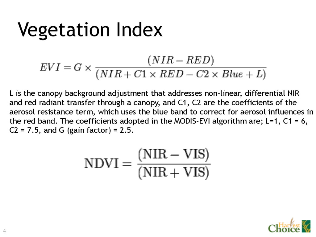
4. Vegetation Index 4 L is the canopy background adjustment that addresses non-linear, differential NIR and red radiant transfer through a canopy, and C1, C2 are the coefficients of the aerosol resistance term, which uses the blue band to correct for aerosol influences in the red band. The coefficients adopted in the MODIS-EVI algorithm are; L=1, C1 = 6, C2 = 7.5, and G (gain factor) = 2.5.
5. Satellite MODIS AVHRR Product MOD13A2 NDVI-g Vegetation Index EVI NDVI Temeroal resolution 16 days 10 days Spatial resolution 1 sqkm 8 sqkm Data availability 2000 – 2012* 1981-2009* Product
6. Ve get ati on Ind ex (sc ale d) Time Season I Season II Original data Fitted data (Savitsky- Golay) Brown dots are: Start of the season, max of the growing season, end of season Method
7. Ve get ati on Ind ex (sc ale d) Time Season I Season II Method
8. Outputs ▪ Vegetation intensity (Single, double, triple seasons) ▪ Starts of the growing dates ▪ Ends of the growing dates ▪ Length of growth periods ▪ Temporal dynamics of vegetation phenology ▪ Trend analysis 8
9. Overview ! ▪ Mapping vegetation phenology and more ▪ Travel time to cities 2010-2012 ▪ Spatial production allocation model (SPAM) 2005 ▪ Tools and apps 9
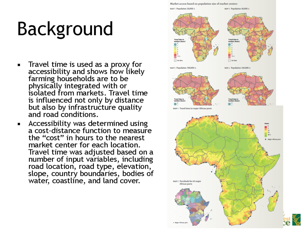
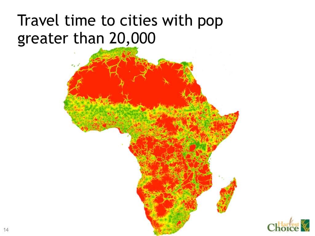
10. Background ▪ Travel time is used as a proxy for accessibility and shows how likely farming households are to be physically integrated with or isolated from markets. Travel time is influenced not only by distance but also by infrastructure quality and road conditions. ▪ Accessibility was determined using a cost-distance function to measure the “cost” in hours to the nearest market center for each location. Travel time was adjusted based on a number of input variables, including road location, road type, elevation, slope, country boundaries, bodies of water, coastline, and land cover.
11. Potential issues ▪ Input data could be outdates since most of the measurement are based on ~2000. (e.g. land cover, settlements/cities, road networks) ▪ Resolution could be coarser for contain country or regional studies. ▪ Not fully harmonized with potential spatial datasets (new roads, different road attributes). ▪ Some parameters of the model need to be improved and refined. ▪ crowdsourcing
12. Updates 2010 version (Africa Only) • Road networks ( road networks are updating to for Mali, Kenya, Malawi, Senegal, Uganda, Nigeria, Tanzania, Burundi, Ethiopia, Ghana, ) • Land cover (2009 data with more details land cover classes following LCCS systems and higher spatial resolution) • Human settlements ( 2010 and harmonize across different sources) • Fine tune model parameters
13. Examples 13 MapCode Global legend without biome separation (Level 1) Regional legend without biome separation (Level 2) A11 - Cultivated Terrestrial Areas and Managed Lands A11 - Cultivated Terrestrial Areas and Managed Lands 10 Cultivated and Managed areas 11 Post-flooding or irrigated croplands (or aquatic) 12 Post-flooding or irrigated shrub or tree crops 13 Post-flooding or irrigated herbaceous crops 14 Rainfed croplands 15 Rainfed herbaceous crops 16 Rainfed shrub or tree crops (cashcrops, vineyards, olive tree, orchards,…) 20 Mosaic cropland (50-70%) / vegetation (grassland/shrubland/forest) (20-50%) 21 Mosaic cropland (50-70%) / grassland or shrubland (20-50%) 22 Mosaic cropland (50-70%) / forest (20-50%) 30 Mosaic vegetation (grassland/shrubland/forest) (50-70%) / cropland (20-50%) 31 Mosaic grassland or shrubland (50-70%) / cropland (20-50%) 32 Mosaic forest (50-70%) / cropland (20-50%)
14. 14 Travel time to cities with pop greater than 20,000
15. Overview ! ▪ Mapping vegetation phenology and more ▪ Travel time to cities 2010-2012 ▪ Spatial production allocation model (SPAM) 2005 ▪ Tools and apps 15
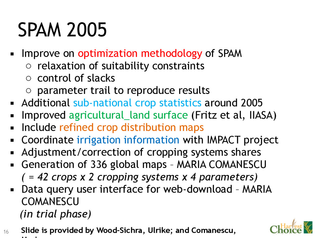
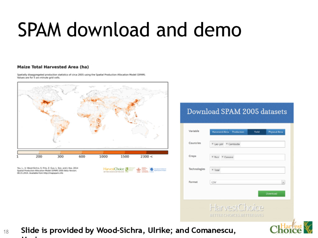
16. SPAM 2005 16 ▪ Improve on optimization methodology of SPAM o relaxation of suitability constraints o control of slacks o parameter trail to reproduce results ▪ Additional sub-national crop statistics around 2005 ▪ Improved agricultural_land surface (Fritz et al, IIASA) ▪ Include refined crop distribution maps ▪ Coordinate irrigation information with IMPACT project ▪ Adjustment/correction of cropping systems shares ▪ Generation of 336 global maps – MARIA COMANESCU ( = 42 crops x 2 cropping systems x 4 parameters) ▪ Data query user interface for web-download – MARIA COMANESCU (in trial phase) Slide is provided by Wood-Sichra, Ulrike; and Comanescu,
17. Overview ! ▪ Mapping vegetation phenology and more ▪ Travel time to cities 2010-2012 ▪ Spatial production allocation model (SPAM) 2005 ▪ Tools and apps 17
18. SPAM download and demo 18 Slide is provided by Wood-Sichra, Ulrike; and Comanescu,
19. AfricaRISING: Project Mapping and 
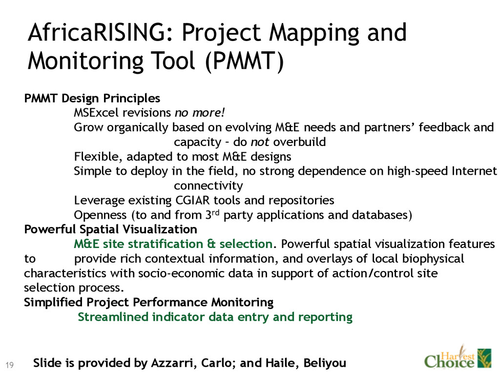
 Monitoring Tool (PMMT) 19 PMMT Design Principles MSExcel revisions no more! Grow organically based on evolving M&E needs and partners’ feedback and capacity – do not overbuild Flexible, adapted to most M&E designs Simple to deploy in the field, no strong dependence on high-speed Internet connectivity Leverage existing CGIAR tools and repositories Openness (to and from 3rd party applications and databases) Powerful Spatial Visualization M&E site stratification & selection. Powerful spatial visualization features to provide rich contextual information, and overlays of local biophysical characteristics with socio-economic data in support of action/control site selection process. Simplified Project Performance Monitoring Streamlined indicator data entry and reporting Slide is provided by Azzarri, Carlo; and Haile, Beliyou
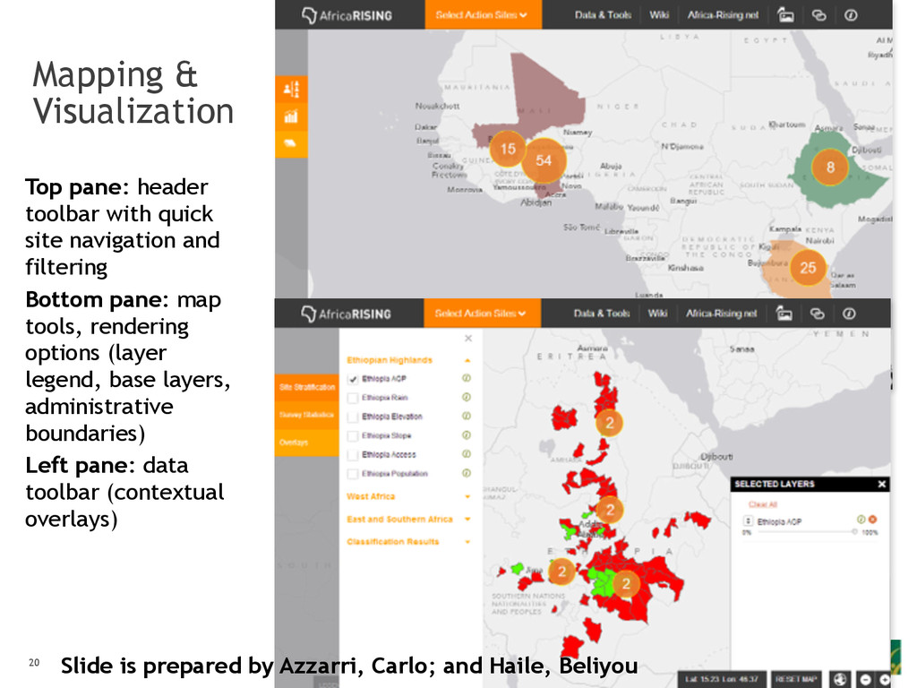
20. 20 Mapping & Visualization Top pane: header toolbar with quick site navigation and filtering Bottom pane: map tools, rendering options (layer legend, base layers, administrative boundaries) Left pane: data toolbar (contextual overlays) Map: Africa RISING megasites and community clusters. Slide is prepared by Azzarri, Carlo; and Haile, Beliyou