A journey through the scientific python ecosystem

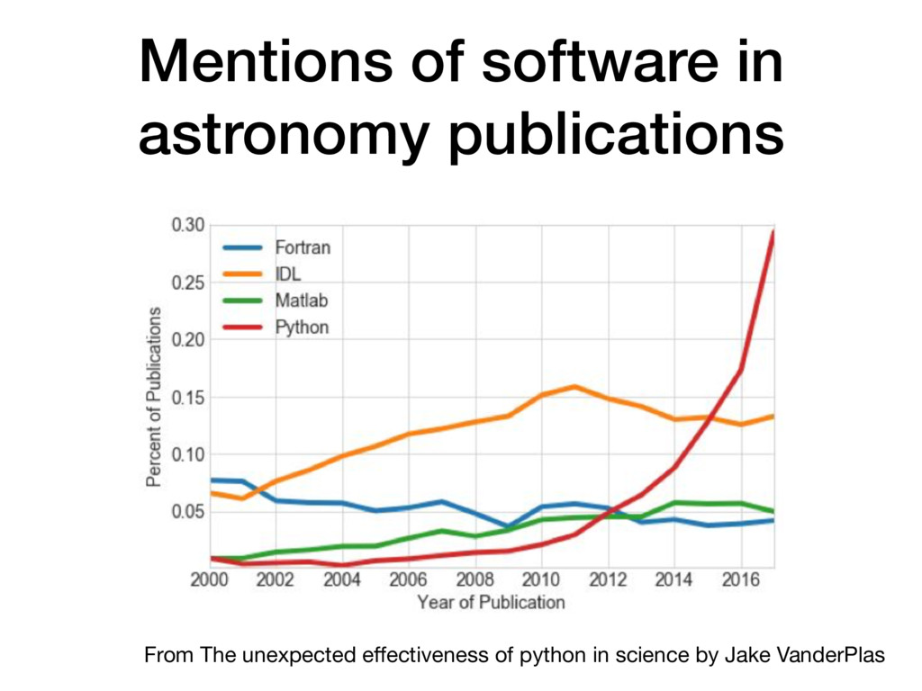
Today, python's use for science is pervasive, in domains as different as astrophysics, neuroscience, or econometrics. Realistically, writing code has become an essential part of most scientists' job. The goal of this talk is to explain why python became successful in science even though it is a generic programming language, and convince the non programmers that they can benefit from using some python in their scientific endeavor as well.

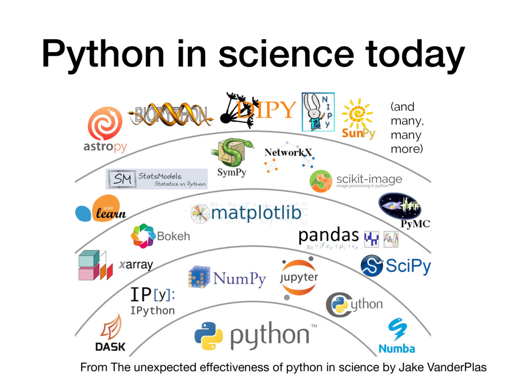
After giving an overview of the main tools available in the scientific
python ecosystem, I will give some concrete examples of simple tasks that can be fastidious but solved quickly with just a bit of python code, from data handling to data visualization.

Transcript

1. A journey through the scientific python ecosystem David Cournapeau @cournape
2. • Notes: • This presentation took a lot of inspiration from “the unexpected effectiveness of python in science” by Jake VanderPlas
3. Who am I • I am David Cournapeau, cournape on twitter/github/ stackoverflow
4. Where I come from • Strasbourg, France
5. Me on the internet • Code • (mostly in the past)
6. Me at work • Cogent Labs: https:// www.cogent.co.jp • We are applying AI/Deep Learning to difficult business problems: • Handwriting recognition (tegaki.ai) • Language understanding (kaidoku) • Time series analysis (finance, etc.) • We are hiring: experience software engineers, ML engineers, Research Scientists in DL/statistics
7. A bit of history
8. My journey to python • Started using python around 2005 for audio processing • Heavy Matlab user at that time • Hit limitations of matlab/C integration • Built a hodgepodge of Matlab, C, python and hdf5 for data transfer • Python was easy to integrate with C, had libraries to parse XML, audio files, do complex GUI, etc.
10. This was typical “Scientists... work with a wide variety of systems ranging from simulation codes, data analysis packages, databases, visualization tools, and home-grown software-each of which presents the user with a different set of interfaces and file formats. As a result, a scientist may spend a considerable amount of time simply trying to get all of these components to work together in some manner...” By David Beazley Scientific Computing with Python In ASP Conf. Ser., Vol. 216, ADASS
11. Python as a glue language • As python could replace bash, sed/awk, and also call into other programs, python became an increasingly popular choice in the 90ies as a glue language • It was also “easy” to interface with C and Fortran libraries • But python was not the only such language: Perl, Tcl/TK, GNU guile or ruby • Something else needed to happen
12. Array computing • At the lowest level, lots of scientific work is about numerical computation • They need to be efficient • People in the 90ies work on array computing in python (matrix-sig) • Matrix package by Jim Fulton, extended by Jim Hugunin -> become Numeric • Paul Dubois, Konrad Hinsen, David Ascher, Travis Oliphant and other continue that work • “grand unification” into NumPy around 2005
13. “Exploratory computing” • IPython started around 2000 by Fernando Perez: python shell optimized for exploratory scientific work • Matplotlib started around 2000 by late John Hunter
14. Mentions of software in astronomy publications From The unexpected effectiveness of python in science by Jake VanderPlas
15. Python as a language for science • Its main strengths come from being a general programming language • Benefit from a large community outside scientists • Also its main weaknesses: • Not integrated (no “python IDE with everything in it”) • Can be confusing for new comers
16. Python in science today Python’s Scientific Ecosystem (and many, many more) Bokeh From The unexpected effectiveness of python in science by Jake VanderPlas
17. A brief tour
18. Installing python 1. Use what your colleagues use 2. Otherwise, use one of the binary distribution available: anaconda, canopy, python(x, y), etc. 3. People with more experience at the command line: `python -m pip —user install …`
19. Pandas: “excel in python” • Pandas is a library for labeled data: ideal for time series, csv, data cleaning, etc… import numpy as np import pandas as pd df = pd.DataFrame( {“normal_1": np.random.randn(1024), "normal_2": np.random.randn(1024) + 5}) df.hist(bins=50)
20. Pandas: example ED normalized_ED count Error_distribution field_type field_name 1.057 0.150 174 [0.575 0.144 0.132 0.046 0.034 0.040 0.029 0.000] sentence form1/fields/69 0.914 0.344 174 [0.316 0.500 0.155 0.017 0.006 0.006 0.000 0.000] sentence form1/fields/31 import pandas as pd df = pd.read_table("report.txt") print("columns: {}".format(", ".join(df.columns))) print("Total count: {}".format(df["count"].sum())) print("Average of normalized ED: {}".format((df["count"] * df["normalized_ED"]).sum() / df["count"].sum())) columns: ED, normalized_ED, count, Error_distribution, field_type, field_name Total count: 7479 Average of normalized ED: 0.17594825511432008
21. When to use pandas • Use pandas when you need to munge / plot data quickly • Can often replace simple use cases of excel (plot, pivoting, aggregation, etc.), but in a more manageable manner
22. Numerical computations • NumPy: the backbone of scientific computing in python • Provides the ndarray object for efficient manipulation of data arrays import numpy as np x = np.random.randn(1024) y = 0.1 * np.random.randn(1024) + 5 # for every 0 <= i < 1024, z[i] = x[i] + y[i] z = x + y
23. Vectorization • Key to good performances in NumPy is to use vectorization • If vectorization too difficult: look at numba, cython import numpy as np def naive_version(x, y): s = 0 for i in range(len(x)): s += x[i] * y[i] return s def numpy_version(x, y): return np.sum(x * y) x = np.random.randn(int(1e6)) y = np.random.randn(int(1e6)) In [6]: %timeit naive_version(x, y) 276 ms ± 8.95 ms per loop (mean ± std. dev.) In [7]: %timeit numpy_version(x, y) 3.01 ms ± 51.5 µs per loop (mean ± std. dev.) ~NumPy 90x faster !
24. When to use NumPy • The common data array structure used by most scientific libraries • If you are new to python, or deals with time-series, or comes from R, or uses excel a lot: starts with pandas • If you are more experienced, and/or doing numerical computing, machine learning, etc.: maybe starts with NumPy
25. Matplotlib • Was initially designed as a replacement for Matlab for plotting import numpy as np import matplotlib.pyplot as plt x = np.linspace(0, 10, 1000) # Noisy sinusoid y = np.sin(x) + 0.1 * np.random.randn(len(x)) plt.plot(x, y)
26. Visualization with pandas • Pandas provide shortcuts for simple plots through matplotlib import pandas as pd data = pd.read_csv('iris.csv') data.plot.scatter( ‘PetalLength', 'PetalWidth')
27. Seaborn • Seaborn is built on top of matplotlib, for statistical plots import pandas as pd import seaborn data = pd.read_csv('iris.csv') seaborn.pairplot(data, hue='Name')
28. Other visualization libraries • Visualization landscape is changing rapidly • I am not a specialist in viz • Recent libraries focus on: • visualization of large datasets • web-based interfaces • Examples: bokeh, plotly, plotnine
29. Bokeh: interactive plotting in the browser From bokeh website
30. Plotly: modern platform for data science From plotly website
31. scikit-learn: machine learning in python • Provides many recent Machine Learning algorithms, under a common API • Appropriate for many classification problems • Can be used for unsupervised classification as well • Some algorithms have online versions as well (for out of core computation, see also dask) • But: • Purposely does not handle complex neural networks (no GPU support, etc.) • API does not fit every ML problem
32. Scikit-learn: example import numpy as np import matplotlib.pyplot as plt from sklearn.ensemble import RandomForestRegressor x = 10 * np.random.rand(100) y = np.sin(x) + 0.1 * np.random.randn(100) model = RandomForestRegressor() model.fit(x[:, np.newaxis], y) xfit = np.linspace(-1, 11, 1000) yfit = model.predict(xfit[:, np.newaxis]) plt.plot(x, y, '.k') plt.plot(xfit, yfit)
33. Scikit-learn: example import numpy as np import matplotlib.pyplot as plt from sklearn.svm import SVR x = 10 * np.random.rand(100) y = np.sin(x) + 0.1 * np.random.randn(100) model = SVR() model.fit(x[:, np.newaxis], y) xfit = np.linspace(-1, 11, 1000) yfit = model.predict(xfit[:, np.newaxis]) plt.plot(x, y, '.k') plt.plot(xfit, yfit)
34. Numba: accelerate numeric python • Numba can be used to optimize python code. • More specialized than general JIT python interpreters (is e.g. pypy) • Designed to run within standard CPython import numpy as np import numba @numba.jit def naive_version(x, y): s = 0 for i in range(len(x)): s += x[i] * y[i] return s def numpy_version(x, y): return np.sum(x * y) x = np.random.randn(int(1e6)) y = np.random.randn(int(1e6)) In [2]: %timeit numpy_version(x, y) 1.73 ms ± 46.2 µs per loop (mean ± std. dev.) In [3]: %timeit naive_version(x, y) 1.22 ms ± 29.1 µs per loop (mean ± std. dev.) Faster than NumPy !
35. Misc • For performance, look at cython and numba • For statistics, look at statsmodels (e.g. TimeSeries model like ARIMA, etc.) • For Deep Learning: very rapidly changing ecosystem (tensorflow, keras, pytorch, dynet, etc.) • For image processing: scikit-images
36. Thank you ! • On github: https://github.com/cournape • On Twitter: https://twitter.com/cournape • I will be there at the party tonight if you want to chat !