The Progenitors of Dwarf Galaxies in Galaxy Clusters

Talk discussing how Luminous Compact Blue Galaxies at intermediate redshifts are likely to evolve into dwarf elliptical galaxies in clusters. Present at http://clusters2017.wixsite.com/cl2017

Transcript

1. The Progenitors of Dwarf Galaxies in Galaxy Clusters Steve Crawford @astrocrawford South African Astronomical Observatory Collaborators: Matthew Bershady (U. Wisconsin), Greg Wirth (Keck Observatory), Solohery Randriamampandry (U. KwaZulu-Natal)
2. Overview • Connecting populations • Luminous Compact Blue Galaxies are triggered in galaxy clusters • LCBGs have similar properties as dE • Fate of LCBGs
3. Dwarf Ellipticals in clusters Jerjen A. Moretti et al.: Galaxy Luminosity Functions in WINGS clusters Fig. 8. Composite Luminosity Function of WINGS galaxies Superimposed are the double Schechter fits obtained having im posed the bright end slope αf = −1.10: red for the population of galaxies, green for the population of galaxies and unknown The two insets in the lower right corner are the values of the fit The black lines are fits taken from the literature (see the top lef inset). Moretti et al. 2015 Dwarf Ellipticals are heterogeneous class that is the most numerous in clusters
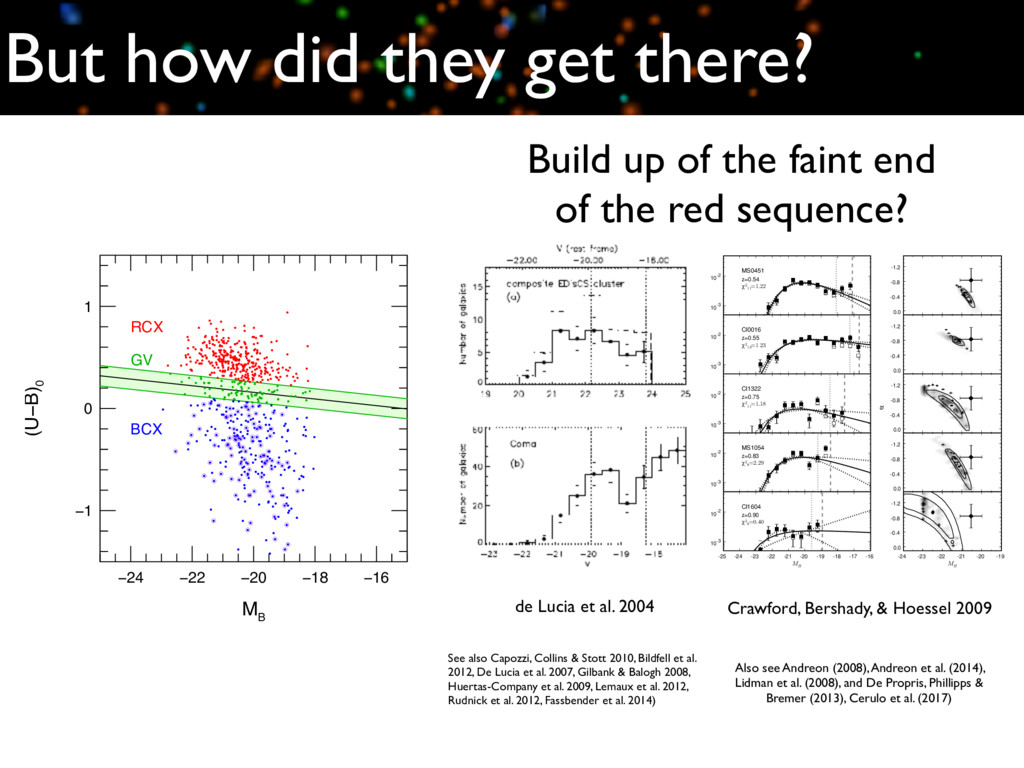
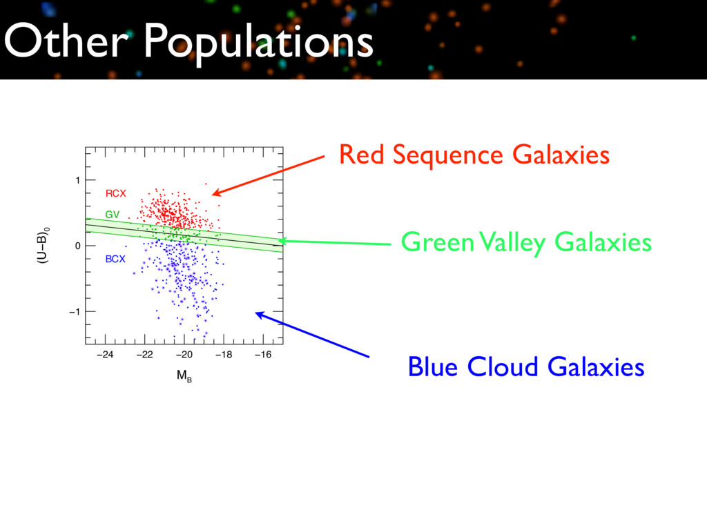
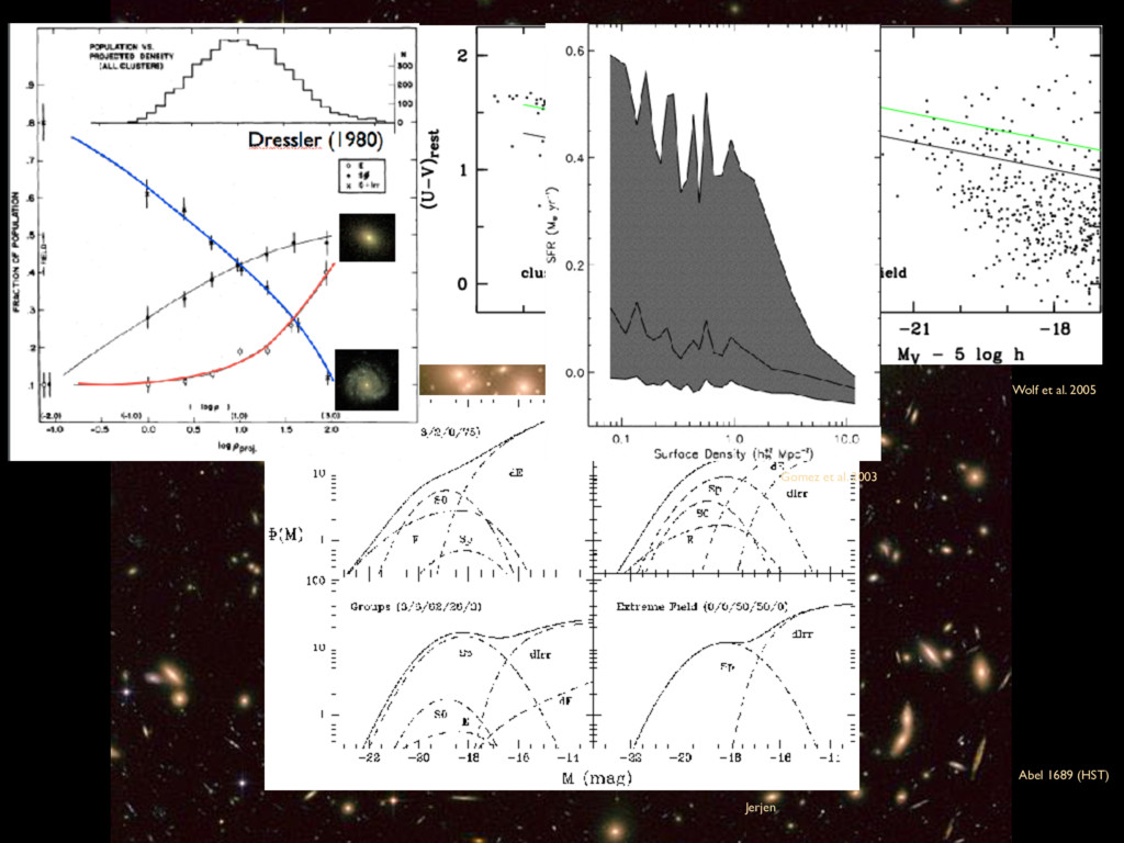
4. But how did they get there? de Lucia et al. 2004 See also Capozzi, Collins & Stott 2010, Bildfell et al. 2012, De Lucia et al. 2007, Gilbank & Balogh 2008, Huertas-Company et al. 2009, Lemaux et al. 2012, Rudnick et al. 2012, Fassbender et al. 2014) 1164 CRAWFORD, BERSHADY, & HOESSEL Vol. 690 10-3 10-2 Cl0016 z=0.55 3 1 3 2 . 1 = 2 χ -1.2 -0.8 -0.4 0.0 10-3 10-2 MS0451 z=0.54 1 1 2 2 . 1 = 2 χ -1.2 -0.8 -0.4 0.0 10-3 10-2 MS1054 z=0.83 8 9 2 . 2 = 2 χ -1.2 -0.8 -0.4 0.0 10-3 10-2 0 0 2 ] −3 c p M [ ) R < ( Cl1322 z=0.75 1 1 8 1 . 1 = 2 χ -1.2 -0.8 -0.4 0.0 -25 -24 -23 -22 -21 -20 -19 -18 -17 -16 B M 10-3 10-2 Cl1604 z=0.90 8 0 4 . 0 = 2 χ -24 -23 -22 -21 -20 -19 B M -1.2 -0.8 -0.4 0.0 Figure 7. Left: RSLF within R200 in each of our five clusters. The open squares represent raw counts; the solid squares are the counts after all corrections (see the text). The best-fit LF are solid black lines, with 68% confidence limits as gray dotted lines. The best-fit χ2 ν and dof is given in each frame. The 50% and 90% completeness limits are plotted as heavy dashed and dotted lines. Right: error ellipses (65% and 95%) are plotted for α and M∗ based on the χ2 distribution. The best-fit value for data down to the 50% and 90% detection-completeness limit are plotted as solid and open circles, respectively. Best-fit values for 10 realizations of the photometry with √ 2 larger errors are plotted as plus symbols (see the text). The gray scale represents results from jack-knife estimates of the errors. We also plot the best-fit value from the low-redshift cluster sample within R200. results and those for R200 are shown in Figure 8 and listed in Table 2. 3.1.1. Trends with Selection Radius Substantial differences in the shape of the LF are seen at smaller selection radii, consistent with local clusters (Lobo et al. 1997; Popesso et al. 2006), and presumably due to a morphology–density relation in the DGR. This effect is illustrated in our study in Figure 8. Our clusters show a general trend of a flatter (α ∼ −1) LF with increasing cluster radius, albeit with significant scatter, especially for Cl1322 and Cl1604, where our errors are largest. In the literature, Lobo et al. (1997) find a steeper faint-end slope in the central regions of Coma as compared to groups around the outskirts. Popesso et al. (2006) Crawford, Bershady, & Hoessel 2009 Also see Andreon (2008), Andreon et al. (2014), Lidman et al. (2008), and De Propris, Phillipps & Bremer (2013), Cerulo et al. (2017) −24 −22 −20 −18 −16 −1 0 1 M B (U−B) 0 RCX GV BCX −.5 0 .5 1 1.5 26 24 22 20 18 16 (B−V) 0 µ e (B) 0 LCBG Build up of the faint end of the red sequence?
5. Blue fraction Butchler & Oemler 1984 Haines et al. 2009
6. LCBGs −16 −.5 0 .5 1 1.5 26 24 22 20 18 16 (B−V) 0 µ e (B) 0 LCBG Luminous Compact Blue Galaxies ompact Blue axies • Original discovered by Koo & Kron in 80s as an observational class: unresolved blue galaxies • Rapidly evolution heterogeneous population of galaxies (factor of ~10 drop since z~1, Guzman et al. 1997) • Luminous (MB ~ -20), small (re ~2 kpc), and intense star formation rates Ref: Koo et al. 1994, Koo et al. 1997, Guzman et al. 1996; Phillips et al. 1997; Kobulnicky & Zaritsky 1999; Guzma ́n et al. 2003; Garland et al. 2004; Werk et al. 2004; Barton et al. 2006; Noeske et al. 2006; Rawat et al. 2007; Hoyos et al. 2007; Tollerud et al. 2010 HST/WFPC2/NICMOS
7. LCBG are like ... Low-z Cardamone et al. 2009 Burgarella et al. 2009 High-z Blue Compact Dwarfs, HII galaxies Lyman Break Galaxies green peas Int-z <3.5 Gyrs ago Up to 3.5-9 Gyrs ago >9 Gyrs ago Extreme Emission Line Galaxies CNELGs z < 0.3 0.3 < z < 1 z>1
8. LCBGs in Clusters Handful of LCBGs in CL0024 seem to have similar properties to low redshift dwarf galaxies Koo original proposed LCBGs as the progenitors of dE Koo et al. 1994
9. Observations Deep WIYN narrow band imaging combined with DEIMOS spectra, Archive HST, Spitzer, and VLA observations
10. Identifying Cluster LCBGs ~15-35% of z=0.5-0.9 cluster galaxies are LCBGs Color key: Red Sequence Galaxies Green Valley Galaxies Blue Cloud Galaxies Luminous Compact Blue Galaxies Crawford et al. 2011, 2014
11. “Shell-like” LCBG Radial Distribution Similar to results for low-z SF galaxies e.g. Thompson 1986; Ellingson et al. 2001; Mahajan et al. 2010 Crawford et al. 2011, 2014
12. LCBGs are falling into the cluster Crawford et al. 2014
13. Clusters Triggering LCBGs Density of Cluster Galaxies Density of field galaxies Enhancement = Enhancement of LCBGs arison between giant galaxies, iral galaxies enhancement imilar to dE or ype galaxy. cantly different e spiral ution. Crawford et al. 2006, 2011
14. Young burst in dE Rys et al. 2015 Rys et al. showed that the typical dE had a burst of star formation ~5 Gyrs ago Also see Michielson et al 08, Lelli et al. 2014, Toloba et al. 2014, Mentz et al 2016
15. Bursts in Illustris Simulations 8 Mistani et al. 2 4 6 8 10 12 0.0 0.5 1.0 1.5 2.0 2.5 SFR [M /yr] SFR =1.68 < SFR > Satellite A 2 4 6 8 10 12 SFR =2.20 Satellite B 2 4 6 8 10 12 t [Gyr] SFR =0.67 Satellite C 2 4 6 8 10 12 SFR =0.66 Satellite D 2 4 6 8 10 12 SFR =0.73 Field Figure 7. Examples of individual star formation histories for the same satellite and field dwarfs in Fig. 3. As in the case of the orbits, the SFR histories of cluster dwarfs exhibit large variations. It is not uncommon to see “peaks” or episodes of intense star formation (for example Sat. A, B) that coincide with the crossing of the virial radius of the cluster and/or first pericentric passages. Starburst events are not common for field dwarfs. Some cluster dwarfs show a more constant SFR that is comparable to field objects (for example Sat. D). In each panel, we quote the “starburstiness” of the curve, SFR , defined as the standard deviation of the SFR history with respect to the time-average h SFR i (cyan line). Large values of h SFR i indicate the presence of starbursts. (See text for more details.) Mistani et al. 2015 Dwarfs galaxies undergo a burst when entering the cluster
16. Spectroscopic Properties – 19 – Fig. 3.— Comparison between the size, absolute magnitude, mass, and star formation rate Cluster and field LCBGs nearly indistinguishable in terms of dynamical mass, SFR, abundance, or size. Typical properties: σ~56 km/s, r1/2~1.8 kpc Mdyn~5x109 M⊙ 12 + log(O/H) = 8.6. Crawford et al. 2016
17. Spectroscopic Properties NGC 205 — local dwarf Elliptical Crawford et al. 2016 Distribution of cluster dE
18. Dynamical to Stellar Mass 8 S. M. Randriamampandry et al. Figure 4. Comparison of best-fit BC03 stellar masses (M⇤) and dynamical masses (Mdyn) of cluster LCBGs (teal circles) to the field sample (grey triangles). The black dashed line indicates the sample. The distribution of the ratios is presented right-hand panel of Figure 3. While the K-S test d rule out the null hypothesis, a random sampling of values only reproduces the median cluster value in the samples. We find that the baryonic mass exceeds the d cal mass (i.e., M⇤ > Mdyn) for several targets. In our sample, for which we have derived measurements erro one galaxy has a baryonic mass greater than the dy mass by more than 1 (standard error). We interp as indicating existence of relatively modest systemat in our mass estimates. On the other hand, galaxies dominated by dark matter will have a typical upp on the ratio of stellar to dynamical mass of Mdyn/M (i.e., Mdyn 3.3 M⇤) (Peralta de Arriba et al. 2014). the field sample is above this limit while only a few sources show so a high ratio. This further supports clusion of di↵erence in the dynamical to stellar mas of the two populations. 4.1.2 Specific Star Formation Rate Figure 5 shows the specific star formation rate (sS fined as the star formation rate per unit mass) ver lar mass. The star formation rate is measured fr Stellar and Dynamical Masses of Cluster LCBGs at z ⇠ 0.54 7 ystematic and random e↵ects (e.g., photo- completeness in the models, and more com- ion histories) may contribute an additional ainty for which we have not accounted (see 2001; Bundy et al. 2005). However, since ay a↵ect the field sample such systematics cance for our relative comparison. ction of the objects in our sample (⇠ 40%) tisfactory SED fits, producing reduced 2 > s suggests a poor match between the best- ur photometric measurements, causes may erestimated random errors in the photom- atic errors in the photometry (background contamination from emission lines, (d) in- the stellar libraries, and (e) poor choices for rs (Z, dust extinction, and IMF). ly, we lack 2 values for the fits that 2003) achieved with their field LCBG sam- as our primary point of comparison. Given mass errors appear comparable to theirs, we eject any of our galaxies with fits that yield However, to confirm data quality we visually to all our targets and defined a“good”fit as acceptable agreement in at least four filter etained the objects that did not meet this icate their stellar masses as upper limits (<) res A1,A2,A3,A4 show all of the observed model SEDs for our sample. Figure 3. Left: Histogram of cluster (teal) and field (grey) LCBGs dynamical masses. Center: Histogram of cluster and field LCBGs stellar masses using best-fit BC03 values. We find no strong evidence suggesting a significant di↵erence between the two distributions as described in the text. Right: Histogram of the ratio of dynamical-to-stellar mass. LCBG Mdyn/M* Cluster~ 2.6 Field ~ 4.8 Randriamapandry et al. 2017 https://arxiv.org/abs/1706.04534 dE Mdyn/M* Cluster~ 2.2 Field ~ 5.1 Penny et al. 2015
19. “Longitudinal Study” Cluster and Field Dwarfs in Illustris 0 500 1000 1500 2000 2500 r [kpc] Satellite A Satellite B Satellite C Satellite D Field 2 4 6 8 10 12 108 109 1010 Mass [M ] 2 4 6 8 10 12 2 4 6 8 10 12 t [Gyr] 2 4 6 8 10 12 2 4 6 8 10 12 Stellar Mass Gas Mass DM Mass Total Mass Figure 3. Examples of the orbits (top row) and mass evolution (bottom row) of cluster dwarfs (Satellites A-D) and a field dwarf (rightmost column). Or show a wide diversity, with some dwarfs completing more than 3-4 revolutions around the cluster (example Sat. A) and others only recently arriving ( D). The time evolution of the host cluster’s virial radius r 200 are indicated with a black dashed line in each panel. The time of maximum total mass green-dotted line in the bottom row) is indicated in all panels with a vertical dotted line. This time corresponds roughly to the moment they stopped be centrals to become satellites; which can happen right before crossing the virial radius of the cluster like in Sat. A, B and D, or before, if they were accreted a smaller group first and then entered the cluster (like Sat. C). The mass evolution in the bottom row shows clear correlations with the orbits, with a decreas mass after infall as well as close pericentric passages. Tidal stripping is not strong for the stellar component (solid red), although dwarfs in tightly bound or can experience significant stellar mass loss (example Sat. A). Small vertical arrows show the times at which each component (dark-matter, stars, gas) reac its maximum. Stars continue to build up after infall, as shown by the shift between the dotted vertical line and the red arrows. Note that for field dwarfs, wh are not exposed to stripping, the mass in all components peaks only at the present time. Mistani et al. 2015 Simulated Observed
20. Fate of LCBGs Local cluster dE LF 30-75% of dE went through an LCBG phase between z=0.3-1 Crawford et al. 2016
21. Summary • Galaxy Clusters trigger the star burst phase in inflating dwarf galaxies at intermediate redshifts • Spectral properties of LCBGs are very similar to local, cluster dE • Likely between 30-75% of dE experienced a LCBG phase in the last 7.5 Gyrs • Further work needed to study the evolution in dynamical to stellar mass, morphology/size, and complex star bursts
22. Complex Star formation in LCBGs Range of star formation in different metrics Starbursting galaxies need better modeling Crawford et al. 2016
23. Merging Together ~10% of cluster LCBGs will merge with another galaxy Distance to neighbor velocity difference with neighbor Crawford et al. 2016
24. Magnitude-size – 17 – Crawford et al. 2016
25. Substructure Dressler-Shectman statistic is the classic test for substructure: Calculated as the offset from the cluster mean for the 10 nearest neighbors
26. Different Scales Green valley galaxies show a similar substructure as red sequence galaxies, but LCBGs show a strong peak at small numbers Crawford et al. 2016
27. Other Populations −24 −22 −20 −18 −16 −1 0 1 M B (U−B) 0 RCX GV BCX −.5 0 .5 1 1.5 26 24 22 20 18 16 (B−V) 0 µ e (B) 0 LCBG Red Sequence Galaxies Green Valley Galaxies Blue Cloud Galaxies
28. Abel 1689 (HST) Wolf et al. 2005 Jerjen Gomez et al. 2003