Data Analysis Libraries

1 Copyright (C) 2018 National Institute of Informatics, All rights
reserved. Introduction to Machine Learning Theory for Software Engineers 機械学習概論２（データ分析ライブラリー） Etsuji Nakai ver3.0 2018/06/18

Python Career College Copyright (C) 2018 National Institute of Informatics,
All rights reserved. 2 目次 ▪ データ分析用のPythonライブラリー ▪ NumPy & matplotlib入門 - 関数電卓として利用してみる - NumPyによるベクトルと行列の計算 - 確率分布と乱数の取得 - グラフの描画 ▪ pandas入門 - pandasのデータフレーム - データフレームからのデータ抽出 - その他のデータフレームの操作 ▪ サンプルコードの解説 - 最小二乗法のサンプルコード - パーセプトロンのサンプルコード ▪ 参考資料

All rights reserved. 3 サンプルコードの入手について ▪ 新しく開いたノートブック上で次のコマンドを実行すると、本講義のサンプルノートブックがダウンロードできます。 - 次のコマンドを実行すると、Google Drive に接続するための認証用リンクが表示されます。リンクをクリックして、表示された認証コードをコピー＆ペーストで入力してください。 - 次のコマンドを実行すると、サンプルノートブックが Google Drive に保存されます。 from google.colab import drive drive.mount('/content/gdrive') %%bash cd '/content/gdrive/My Drive/Colab Notebooks' git clone https://github.com/enakai00/numpy-pandas-tutorial リンクをクリックして、ユーザー認証を行う

All rights reserved. 6 NumPy, pandas, matplotlib について ▪ この資料では、主に下記のライブラリーを説明します。 - NumPy : ベクトルや行列の演算の他、主要な数学関数や乱数機能を提供します。 - pandas : Rに類似のデータフレーム（スプレッドシートのように、行／列に属性が付いたデータ構造）を提供します。 - matplotlib : グラフを描画します。 ▪ この資料の説明は、Google Colaboratory での実行を前提とします。 - はじめに下記のコマンドを実行して、必要なモジュールをインポートしてあるものとします。 import numpy as np import matplotlib.pyplot as plt import pandas as pd from pandas import Series, DataFrame

All rights reserved. 9 Pythonによる数値計算 ▪ コードセルに計算式を入力すると、計算結果が表示されます。 - 冪乗は「**」を用います。直前の結果は、「_」で参照できます。 - Python 2 の環境では、小数点以下のない数値は、整数型とみなされます。実数値として計算する場合は、小数点以下を明示するか、float()で実数型に変換します。 • 安全のために（実数として計算したい）数値の末尾には「.0」を付与する習慣を付けておきましょう。 • 実数型と整数型が混在した計算では、実数型として計算が行われます。 In [2]: 2*(1+3) Out[2]: 8 In [3]: 2**10 Out[3]: 1024 In [4]: _ * 2 Out[4]: 2048 In [5]: 1/2 Out[5]: 0.5 In [6]: 1.0/2 Out[6]: 0.5 In [7]: float(1)/2 Out[7]: 0.5 Python 2 の環境では 0 になる

All rights reserved. 10 NumPyが提供する数学関数の利用 ▪ NumPyが提供する各種関数や定数値が利用できます。 - 最初にモジュールをインポートする際に、省略名「np」で参照できるようにしてあります。 - NumPyが提供する関数は、リスト（もしくは、array）を代入すると、それぞれの要素を代入した結果のarrayが返ります。（リストとarrayの違いは、後ほど説明します。） - この性質は、後ほど、関数のグラフを描く際に必要となります。自分で関数を定義する際も、この性質（リストを代入するとarrayが返る）を実装するように心がけましょう。 In [8]: np.pi Out[8]: 3.141592653589793 In [9]: np.e Out[9]: 2.718281828459045 In [10]: np.sin(np.pi/4) Out[10]: 0.70710678118654746 In [11]: np.sqrt(2) Out[11]: 1.4142135623730951 In [12]: np.sqrt([0,1,2,3]) Out[12]: array([ 0. , 1. , 1.41421356, 1.73205081])

All rights reserved. 11 散布図と折れ線グラフ In [13]: data_x = [0.0, -0.95, -0.59, 0.59, 0.95] data_y = [1.0, 0.31, -0.81, -0.81, 0.31] plt.scatter(data_x,data_y) - 散布図は、対象データの「x座標のリスト」と「y座標のリスト」を用意して、plt.scatter()に渡します。「座標(x,y)のリスト」を渡すわけではないので注意してください。 - 折れ線グラフは、対象データの「x座標のリスト」と「y座標のリスト」を用意して、plt.plot()に渡します。 - グラフの見栄えを綺麗にする方法は、後ほど説明します。 In [14]: data_x = [0,1,2,3,4,5] data_y = [0,1,4,9,16,25] plt.plot(data_x,data_y) ▪ matplotlibを用いて、散布図と折れ線グラフを表示してみます。

All rights reserved. 12 散布図と折れ線グラフ - 関数のなめらかなグラフを描く際は、十分に細かく分割した「x座標のリスト」を用意して、対応する「y座標のリスト」を計算します。 - 「x座標のリスト」は、np.linspace()を使って生成すると便利です。「y座標のリスト」（data_y）の計算では、関数にリスト（array）を代入するとarrayが得られる性質を利用しています。 - np.linspace()の代わりに、np.arange()を使用することもできます。 In [15]: data_x = np.linspace(0, 1, 101) data_y = np.sin(2.0*np.pi*data_x) plt.plot(data_x,data_y) [0,1]を100分割した101個の実数を生成 data_x = np.arange(0, 1.01, 0.01)

All rights reserved. 16 行列とベクトルの計算 ▪ 行列／ベクトルは、NumPyのarrayオブジェクトで表現します。 - 2次元リストをnp.array()に渡すと、対応するarrayオブジェクトが得られます。 • 入力セルの最後に変数のみを記載すると、変数の内容が表示されます。 - 通常の2次元リストではできない、行列の積や逆行列などの演算が用意されています。行列の積と逆行列は、それぞれ、np.dot()、np.linalg.inv()で計算します。 - 転置行列は、T属性を用います。 In [2]: theta = np.pi / 3 m = np.array([[np.cos(theta), -np.sin(theta)], [np.sin(theta), np.cos(theta)]]) m Out[2]: array([[ 0.5 , -0.8660254], [ 0.8660254, 0.5 ]]) In [3]: np.dot(m, m) Out[3]: array([[-0.5 , -0.8660254], [ 0.8660254, -0.5 ]]) In [4]: np.linalg.inv(m) Out[4]: array([[ 0.5 , 0.8660254], [-0.8660254, 0.5 ]]) In [5]: m.T Out[5]: array([[ 0.5 , 0.8660254], [-0.8660254, 0.5 ]]) ※ 回転行列について、一般に次の性質が成り立ちます。

All rights reserved. 17 行列とベクトルの計算 - ベクトルは、　　　行列として定義することで、行列との積や内積／外積が計算できます。 - ベクトルの内積とクロス積は次のように計算できます。 ※ ベクトルを1次元リストとして定義した場合の演算ルールについては後ほど説明します。 In [6]: x = np.array([[1], [0]]) x Out[6]: array([[1], [0]]) In [7]: n = np.dot(m, x) n Out[7]: array([[ 0.5 ], [ 0.8660254]]) In [8]: a = np.array([[-1], [0], [1]]) b = np.array([[2], [3], [5]]) np.dot(a.T, b) Out[8]: array([[3]]) In [9]: np.dot(a, b.T) Out[9]: array([[-2, -3, -5], [ 0, 0, 0], [ 2, 3, 5]]) In [10]: np.dot(a.T, b)[0][0] Out[10]: 3 成分指定でスカラーとして取り出す場合

All rights reserved. 18 ブロードキャストルール ▪ スカラー演算をarrayに適用すると、各成分に対する演算が行われます。これをブロードキャストルールと呼びます。 - 行列／ベクトルのスカラー倍は、ブロードキャストルールとして自然に計算されます。 - 次は、数学の演算としては不自然ですが、ブロードキャストルールが適用される例になります。 In [11]: m = np.array([[1,2], [3,4]]) m Out[11]: array([[1, 2], [3, 4]]) In [12]: 2*m Out[12]: array([[2, 4], [6, 8]]) In [13]: m*2 Out[13]: array([[2, 4], [6, 8]]) In [14]: m**2 Out[14]: array([[ 1, 4], [ 9, 16]]) In [15]: m+10 Out[15]: array([[11, 12], [13, 14]]) In [16]: [1, 2, 3] * 2 Out[16]: [1, 2, 3, 1, 2, 3] In [17]: np.array([1, 2, 3]) * 2 Out[17]: array([2, 4, 6]) ※次の計算は、リストとarrayで結果が異なるので　注意してください。

All rights reserved. 19 ブロードキャストルール - ブロードキャストルールを活用すると、リスト／arrayに対して、arrayを返す関数が簡単に作れます。 - 上の例では、リストをarrayに変換していますが、引数は常にarrayで渡すことがわかっている場合、この処理は省略しても構いません。 In [18]: def square(x): if isinstance(x, list): x = np.array(x) return x**2 In [19]: square(3) Out[19]: 9 In [20]: square([1, 2, 3]) Out[20]: array([1, 4, 9]) In [21]: square(np.array([1, 2, 3])) Out[21]: array([1, 4, 9]) In [22]: def square(x): return x**2 square(np.array([1, 2, 3])) Out[22]: array([1, 4, 9])

All rights reserved. 20 ブロードキャストルール ▪ 同じサイズのarray同士のスカラー演算は、対応する成分同士の演算になります。 - 行列の和／差は、自然に計算されます。 - 次のような演算も可能です。 ※ サイズの異なるarray同士のスカラー演算にも、一定の法則でブロードキャストルールが適用されますが、　　直感的にわかりにくい結果になるので、なるべく使用しない方がよいでしょう。 In [23]: a = np.array([[10, 20],[30,4 0]]) a Out[23]: array([[10, 20], [30, 40]]) In [24]: b = np.array([[1, 2], [3, 4]]) b Out[24]: array([[1, 2], [3, 4]]) In [27]: a**b Out[27]: array([[ 10, 400], [ 27000, 2560000]]) In [25]: a+b Out[25]: array([[11, 22], [33, 44]]) In [26]: a-b Out[27]: array([[ 9, 18], [27, 36]])

All rights reserved. 21 arrayオブジェクトの生成と変形 ▪ arrayオブジェクト生成／変形の定番パターンには、次のようなものがあります。 - np.zeros()、np.ones()を用いると、全成分が0、もしくは、1のarrayが得られます。行列サイズを表すタプル (y, x) を引数として渡します。np.eye()は単位行列を生成します。 - 既存のarrayオブジェクトは、reshape()メソッドで縦横のサイズを変更できます。現在のサイズは、shape属性で参照できます。 In [28]: np.zeros((3, 3)) Out[28]: array([[ 0., 0., 0.], [ 0., 0., 0.], [ 0., 0., 0.]]) In [29]: np.ones((2, 3)) Out[29]: array([[ 1., 1., 1.], [ 1., 1., 1.]]) In [31]: a = np.array([1, 2, 3, 4, 5, 6]) a Out[31]: array([1, 2, 3, 4, 5, 6]) In [32]: b = a.reshape((2, 3)) b Out[32]: array([[1, 2, 3], [4, 5, 6]]) In [33]: c = b.reshape((3, 2)) c Out[33]: array([[1, 2], [3, 4], [5, 6]]) In [34]: b.shape Out[34]: (2, 3) In [35]: c.shape Out[35]: (3, 2) In [30]: np.eye(4) Out[30]: array([[ 1., 0., 0., 0.], [ 0., 1., 0., 0.], [ 0., 0., 1., 0.], [ 0., 0., 0., 1.]])

All rights reserved. 22 arrayオブジェクトの生成と変形 - reshape()を用いると、1次元リストを2次元配列としてのベクトルに変換できます。 ※ この変換は次の方法でも可能です。 - 等差数列のarrayは、np.arange()で生成します。np.arange(x, y, s) とした場合、x から y の範囲で公差 s の数列を生成します。終点 y は、数列に含まれない点に注意が必要です。 In [36]: x = [1, 2, 3, 4] np.array(x).reshape(len(x),1) Out[36]: array([[1], [2], [3], [4]]) In [39]: np.arange(0, 1, 0.1) Out[39]: array([ 0. , 0.1, 0.2, 0.3, 0.4, 0.5, 0.6, 0.7, 0.8, 0.9]) In [37]: np.array([x]) Out[37]: array([[1, 2, 3, 4]]) In [38]: np.array([x]).T Out[38]: array([[1], [2], [3], [4]])

All rights reserved. 23 （参考）arrayオブジェクトの生成と変形 - np.vstack()とnp.hstack()は、それぞれ、2つの配列を縦、または、横に結合します。 In [40]: a = np.ones(9).reshape((3, 3)) a Out[40]: array([[ 1., 1., 1.], [ 1., 1., 1.], [ 1., 1., 1.]]) In [41]: b = a*2 b Out[41]: array([[ 2., 2., 2.], [ 2., 2., 2.], [ 2., 2., 2.]]) In [42]: np.vstack((a, b)) Out[42]: array([[ 1., 1., 1.], [ 1., 1., 1.], [ 1., 1., 1.], [ 2., 2., 2.], [ 2., 2., 2.], [ 2., 2., 2.]]) In [43]: np.hstack((a, b)) Out[43]: array([[ 1., 1., 1., 2., 2., 2.], [ 1., 1., 1., 2., 2., 2.], [ 1., 1., 1., 2., 2., 2.]])

All rights reserved. 24 （参考）１次元のarrayに対するnp.dot()の計算 ▪ np.dot()に1次元のarrayを代入した場合は、文脈に合わせて縦ベクトル／横ベクトルの解釈が行われます。 - 1次元arrayどうしは内積になります。 - 2次元arrayと1次元arrayは、行列としての積になります。 ※ 上記以外の組み合わせパターンの場合は、結果が直感とあわない場合もありますので、あまり使用しない方　　がよいでしょう。 In [44]: a = np.array([-1, 0, 1]) b = np.array([ 1, 2, 3]) np.dot(a, b) Out[44]: 2 In [45]: m = np.array([1, 1, 1, 2, 2, 2, 3, 3, 3]).reshape(3, 3) m Out[45]: array([[1, 1, 1], [2, 2, 2], [3, 3, 3]]) In [46]: np.dot(m, a) Out[46]: array([0, 0, 0]) In [47]: np.dot(a, m) Out[47]: array([2, 2, 2])

All rights reserved. 28 一様分布からの乱数の取得 ▪ rand() （numpy.randomモジュールが提供）、および、randint()を用いると、指定範囲の一様な乱数が得られます。また、一度に多数の乱数を生成することができます。 - rand()は、　　　　　の範囲（1は含まない）の実数値の乱数を指定の個数だけ生成します。指定サイズのarrayとして値を返します。 - 同様に、randint()は指定範囲の整数値の乱数を指定の個数だけ生成します。次は、1〜6の範囲（7は含まない点に注意）の乱数を生成する例です。 In [2]: from numpy.random import rand rand() Out[2]: 0.19644145945572267 In [3]: rand(5) Out[3]: array([ 0.64765831, 0.41288461, 0.21530768, 0.3225688 , 0.55119995]) In [4]: rand(2, 3) Out[4]: array([[ 0.63193604, 0.48647432, 0.06980617], [ 0.32513886, 0.29350987, 0.58432974]]) In [5]: from numpy.random import randint Randint(1, 7) Out[5]: 1 In [6]: randint(1, 7,1 0) Out[6]: array([2, 4, 3, 6, 4, 6, 1, 6, 2, 3]) In [7]: randint(1, 7, (3, 5)) Out[7]: array([[3, 1, 3, 1, 5], [2, 5, 5, 1, 1], [1, 3, 6, 5, 2]])

All rights reserved. 29 正規分布からの乱数の取得 ▪ numpy.randomモジュールの normal() を用いると、正規分布からの乱数が得られます。 - 次のように、loc（平均）、scale（標準偏差）、size（arrayのサイズ）を指定します。最後の例のように、パラメータ名を省略しても構いません。 - 1000個の乱数を発生して、ヒストグラムを表示します。 In [8]: from numpy.random import normal normal(loc=0, scale=3, size=10) Out[8]: array([-0.45405421, 1.03407066, -6.06638636, -1.47014096, 2.4127684 , -0.60084586, -2.20008908, -2.49174201, -5.53419474, -2.99053036]) In [9]: normal(loc=0, scale=3, size=(3, 2)) Out[9]: array([[ 4.94332685, -2.65134418], [-5.97073959, -0.94864428], [-1.04192588, 2.29266043]]) In [10]: normal(0, 3, (3, 2)) Out[10]: array([[ 4.55288412, -3.28343893], [ 2.981074 , -2.05497678], [ 0.08205987, 0.77338863]]) In [5]: val = normal(10, 3, size=1000) In [6]: plt.hist(val, bins=20)

All rights reserved. 30 正規分布からの乱数の取得 ▪ numpy.randomモジュールの multivariate_normal() を用いると、多次元の正規分布からの乱数が得られます。 - 次のように、mean（平均）、cov（分散共分散行列）、size（arrayのサイズ）を指定します。パラメータ名は省略しても構いません。 - 200個の乱数を発生して、散布図を表示します。 In [11]: from numpy.random import multivariate_normal c = np.array([[3, 2],[2, 3]]) c Out[11]: array([[3, 2], [2, 3]]) In [12]: multivariate_normal(mean=[50, 10], cov=c, size=4) Out[12]: array([[ 52.09847888, 11.7263966 ], [ 50.72997909, 9.15308538], [ 51.75341106, 11.19224385], [ 48.61627847, 9.09737349]]) In [13]: vals = multivariate_normal([50, 10], c, 200) data_x = [x for (x, y) in vals] data_y = [y for (x, y) in vals] plt.scatter(data_x, data_y)

All rights reserved. 31 同一の乱数を発生する方法 ▪ np.random.seed()で乱数のシード（種）を指定すると、毎回同じ乱数を発生することができます。 - シードの値には、32bit整数を指定します。 In [14]: np.random.seed(10) print (randint(1, 10, 10)) print (randint(1, 10, 10)) Out[14]: [5 1 2 1 2 9 1 9 7 5] [4 1 5 7 9 2 9 5 2 4] In [15]: np.random.seed(10) print (randint(1, 10, 10)) print (randint(1, 10, 10)) Out[15]: [5 1 2 1 2 9 1 9 7 5] [4 1 5 7 9 2 9 5 2 4] シードが同じなので、同じ乱数が発生するシードが同じなので、同じ乱数が発生する

All rights reserved. 36 複数グラフの描画 ▪ 次は、描画ウィンドウを分割して、複数のグラフを並べる際の定番パターンです。 - fig.add_subplot(y, x, c) で取得した描画位置を示すオブジェクト（サブプロット）に対して、 scatter()、plot()などのメソッドを適用します。（描画位置は左上が「1」で、はじめに右に進みます。） - 次は、サブプロットに対して、タイトル、x軸／y軸の描画範囲、x軸／y軸のタイトルを指定する例です。 fig = plt.figure(figsize=(14, 4)) subplot = fig.add_subplot(2, 3, 1) subplot.plot(data1_x, data1_y) subplot = fig.add_subplot(2, 3, 2) subplot.scatter(data2_x, data2_y) 描画ウィンドウのオブジェクトを取得描画ウィンドウを縦2 x 横3 に分割した1つ目の描画位置描画ウィンドウを縦2 x 横3 に分割した2つ目の描画位置１４２５３６ subplot.set_title('ROC graph') subplot.set_xlim([0, 1]) subplot.set_ylim([0, 1]) subplot.set_xlabel("False positive rate") subplot.set_ylabel("True positive rate")

All rights reserved. 39 乱数データの生成とグラフ表示 ▪ 次の条件で乱数データを生成してグラフに表示します。 - 　　　　　の範囲を n 等分したそれぞれの点 x について、正弦関数　　　　　の値に平均 0、標準偏差 0.3 の正規分布ノイズを加えた値 y を生成します。 - 次は、繰り返し処理を用いた、素朴な実装例です。 - 次はブロードキャストルールを利用した実装例です。 from numpy.random import normal def generate_data01(n): data_x = [] data_y = [] for i in range(n): x = float(i) / float(n-1) # [0, 1]をn等分したi番目の値 y = np.sin(2*np.pi*x) + normal(0, 0.3) data_x.append(x) data_y.append(y) return data_x, data_y from numpy.random import normal def generate_data02(n): data_x = np.linspace(0, 1 ,n) # [0, 1]をn等分した値のリスト data_y = np.sin(2*np.pi*data_x) + normal(0, 0.3, n) return data_x, data_y

All rights reserved. 40 乱数データの生成とグラフ表示 ▪ 次のコードを実行すると以下のグラフ表示されます。 - サブプロットオブジェクトに複数のグラフ描画メソッドを適用するとグラフを重ねて表示することができます。 - labelオプションでグラフに付与したラベルは、legend()メソッドで凡例として表示されます。凡例の表示位置（locオプション）については、下記を参照。 • http://matplotlib.org/api/pyplot_api.html#matplotlib.pyplot.legend fig = plt.figure() data_x, data_y = generate_data01(10) #data_x, data_y = generate_data02(10) subplot = fig.add_subplot(1, 1, 1) subplot.set_xlabel('Observation point') subplot.set_ylabel('Value') subplot.set_xlim(-0.05, 1.05) # 生成したデータを表示 subplot.scatter(data_x, data_y, marker='o', color='blue', label='Observed value') # 三角関数の曲線を表示 linex = np.linspace(0, 1, 100) liney = np.sin(2*np.pi*linex) subplot.plot(linex, liney, linestyle='--', color='green', label='Theoretical curve') # 凡例を表示 subplot.legend(loc=1)

All rights reserved. 45 ▪ pandasは、Rのデータフレームとアトミックベクトルに相当するオブジェクトである、 DataFrameとSeriesを提供します。 - DataFrameは、2次元のデータについて行／列のラベルを付与したものです。エクセルシートのように操作することができます。１つの列が１つのデータ項目、１つの行が１つのレコードを表します。 - Seriesは、DataFrameから特定の行、もしくは、列を取り出したものになります。 ▪ 次は、DataFrameの例です。ここでは、各行のラベル（index）は連番、各列のラベル（column）はデータの種類を示す名前として使用しています。 - 各都市の湿度と気温を表にまとめたDataFrame（左図） - 2個のサイコロを振った結果をまとめたDataFrame（右図） DataFrameとSeries

All rights reserved. 46 DataFrameの作成方法 ▪ DataFrameを作成する手順には、次ようなパターンがあります。 - csvファイルからデータを読み込む。 - 各列のデータを表すSeriesオブジェクトを用意して、DataFrameにまとめる。 - データの集合をarrayにまとめておき、DataFrameに変換する。 - columnだけ定義した空のDataFrameを作成して、1行づつデータを加えていく。 - columnすら持たない空のDataFrameを作成して、列を追加していく。

All rights reserved. 47 arrayをDataFrameに変換する方法 ▪ 次は、2次元のarrayをDataFrameに変換する例です。 - columnsオプションで、各列のcolumn名を指定します。 In [2]: from numpy.random import randint dices = randint(1, 7, (5, 2)) dices Out[2]: array([[6, 6], [2, 2], [2, 2], [1, 5], [6, 2]]) In [3]: diceroll = DataFrame(dices, columns=['dice1', 'dice2']) diceroll Out[3]:

All rights reserved. 48 Seriesオブジェクトをまとめる方法 ▪ 次は、SeriesオブジェクトからDataFrameを作成する例です。 - はじめに、各列のデータに対応するSeriesオブジェクトを作成します。Seriesオブジェクトは、 nameオプションでデータの名前が付与できます。 In [4]: city = Series(['Tokyo', 'Osaka', 'Nagoya', 'Okinawa'], name='City') city Out[4]: 0 Tokyo 1 Osaka 2 Nagoya 3 Okinawa Name: City, dtype: object In [5]: temp = Series([25.0, 28.2, 27.3, 30.9], name='Temperature') temp Out[5]: 0 25.0 1 28.2 2 27.3 3 30.9 Name: Temperature, dtype: float64 In [6]: humid = Series([44, 42, np.nan, 62], name='Humidity') humid Out[6]: 0 44 1 42 2 NaN 3 62 Name: Humidity, dtype: float64 np.nanは欠損値を表すダミーデータです。

All rights reserved. 49 Seriesオブジェクトをまとめる方法 - 各列のcolumn名と対応するSeriesオブジェクトのディクショナリを与えて、DataFrameを生成します。 - Seriesオブジェクトの代わりに、リストを用いてもDataFrameを生成することができます。 In [7]: cities = DataFrame({'City':city, 'Temperature':temp, 'Humidity':humid}) cities Out[7]: In [8]: data = {'City': ['Tokyo', 'Osaka', 'Nagoya', 'Okinawa'], 'Temperature': [25.0, 28.2, 27.3, 30.9], 'Humidity': [44, 42, np.nan, 62]} cities = DataFrame(data) Out[8]:

All rights reserved. 50 空のDataFrameに行を追加していく方法 ▪ 次は、空のDataFrameに行を追加する例です。 - はじめに、column名だけを指定したDataFrameを作成します。 - 追加するデータをSeriesオブジェクトとして用意します。この際、indexオプションで、column 名に対応する名前を付けておきます。 - 用意したDataFrameのappend()メソッドで、Seriesオブジェクトを追加します。（Seriesオブジェクトを追加する際は、ignore_index=Trueを指定します。） In [9]: diceroll = DataFrame(columns=['dice1', 'dice2']) diceroll Out[9]: In [10]: oneroll = Series(randint(1, 7, 2), index=['dice1', 'dice2']) oneroll Out[10]: dice1 5 dice2 6 dtype: int64 In [11]: diceroll = diceroll.append(oneroll, ignore_index=True) diceroll Out[11]:

All rights reserved. 51 空のDataFrameに行を追加していく方法 ▪ 次は、2個のサイコロを1000回振った結果をシミュレーションする例です。 - DataFrameのdescribe()メソッドで基本的な統計値を確認することができます。 In [12]: diceroll = DataFrame(columns=['dice1', 'dice2']) for i in range(1000): diceroll = diceroll.append( Series(randint(1, 7, 2), index=['dice1', 'dice2']), ignore_index = True) diceroll[:5] Out[12]: In [13]: diceroll.describe() Out[13]:

All rights reserved. 52 DataFrameを結合する方法 ▪ DataFrameのappend()メソッドは、2つのDataFrameを結合する際にも利用できます。 - ignore_index=Trueを指定すると、indexは通し番号になるように再割当てが行われます。指定がない場合、元のDataFrameのindexが保存されます。 In [14]: diceroll1 = DataFrame(randint(1, 7, (5, 2)), columns=['dice1', 'dice2']) diceroll1 Out[14]: In [15]: diceroll2 = DataFrame(randint(1, 7, (3, 2)), columns=['dice1', 'dice2']) diceroll2 In [16]: diceroll3 = diceroll1.append(diceroll2) diceroll3 Out[16]: In [17]: diceroll4 = diceroll1.append(diceroll2, ignore_index=True) diceroll4 Out[17]: indexを通し番号で採番しなおす。

All rights reserved. 53 DataFrameに列を追加する方法 ▪ 次は、DataFrameに列を追加する例です。 - 配列のindex記法でcolumn名を指定して追加します。（属性で指定する方法は使えません。） - pd.concat()関数で複数のSeriesを列として結合したり、既存のDataFrameにSeriesを列として追加することもできます。 ※ DataFrameの結合方法の全体像については、次のドキュメントを参照　　　　　　　　　　　http://pandas.pydata.org/pandas-docs/stable/merging.html In [18]: diceroll = DataFrame() diceroll['dice1'] = randint(1, 7, 5) diceroll Out[18]: In [19]: diceroll['dice2'] = randint(1, 7, 5) diceroll Out[19]: In [20]: dice1 = Series(randint(1, 7, 5),name='dice1') dice2 = Series(randint(1, 7, 5),name='dice2') diceroll = pd.concat([dice1, dice2], axis=1) diceroll Out[20]: In [21]: dice3 = Series(randint(1, 7, 5), name='dice3') diceroll = pd.concat([diceroll, dice3], axis=1) diceroll Out[21]: 列方向での結合

All rights reserved. 56 列の取り出し ▪ DataFrame から特定の列をSeriesとして取り出します。 - 配列のindexにcolumn名を指定する方法と、column名を属性として指定する方法があります。 ※ 属性として指定する方法は、すこし紛らわしいかも知れません。 In [2]: from numpy.random import randint dices = randint(1, 7 (5, 2)) diceroll = DataFrame(dices, columns=['dice1','dice2']) diceroll Out[2]: In [3]: diceroll['dice1'] Out[3]: 0 5 1 5 2 5 3 6 4 4 Name: dice1, dtype: int64 In [4]: diceroll.dice1 Out[4]: 0 5 1 5 2 5 3 6 4 4 Name: dice1, dtype: int64 配列のindexにcolumn名を指定 column名を属性として指定

All rights reserved. 57 列の取り出し ▪ 複数の列をDataFrameとして取り出すこともできます。 - 配列のindexに複数のcolumn名のリストを指定します。 - 単一の列をSeriesではなく、DataFrameとして取り出す際は次のようにします。 In [5]: data = {'City': ['Tokyo', 'Osaka', 'Nagoya', 'Okinawa'], 'Temperature': [25.0, 28.2, 27.3, 30.9], 'Humidity': [44, 42, np.nan, 62]} cities = DataFrame(data) cities Out[5]: In [6]: cities[['City', 'Humidity']] Out[6]: cities['City', 'Humidity'] ではないので注意 In [7]: cities[['City']] Out[7]: In [8]: cities['City'] Out[8]: 0 Tokyo 1 Osaka 2 Nagoya 3 Okinawa Name: City, dtype: object DataFrameとして取り出し Seriesとして取り出し

All rights reserved. 58 行の取り出し ▪ 行を指定して取り出す際は、配列の「スライス記法」で行を指定します。 - [開始行:終了行-1] で指定します。 - 次のように、特定の条件を満たす行だけを抽出することもできます。 In [9]: cities[0:2] Out[9]: In [10]: cities[2:3] Out[10]: In [11]: cities[1:] Out[11]: In [12]: cities[cities['Temperature']>28] Out[12]:

All rights reserved. 59 行と列を指定した取り出し ▪ 行と列の両方を指定して取り出す際は、loc / iloc メソッドを利用します。 - loc メソッドでは、行と列を名前で指定します。 - iloc メソッドでは、行と列を番号で指定します。 In [13]: cities Out[13]: In [14]: cities.loc[[0, 2], ['City', 'Humidity']] Out[14]: In [15]: cities.iloc[[0, 2], [0, 1]] Out[15]:

All rights reserved. 60 行単位でのIteration処理 ▪ DataFrameの行ごとに処理をする際は、iterrows()メソッドを利用します。 - 各行のindexとその行を表すSeriesオブジェクトが順番に取得できます。 In [16]: cities Out[16]: In [17]: for index, line in cities.iterrows(): print ('Index:', index) print (line, '\n') Index: 0 City Tokyo Humidity 44 Temperature 25 Name: 0, dtype: object Index: 1 City Osaka Humidity 42 Temperature 28.2 Name: 1, dtype: object Index: 2 City Nagoya Humidity NaN Temperature 27.3 Name: 2, dtype: object （・・以下略・・）

All rights reserved. 61 DataFrameから抽出したデータの変更について ▪ これまでに説明した方法でDataFrameから抽出したオブジェクトは、参照専用として扱い、値を変更する操作は行わないでください。 - 抽出方法によって、元のDataFrameのオブジェクトを参照している場合とそうでない場合があり、変更の影響範囲が不明確になります。 - 抽出した方の値を変更する際は、copy()メソッドで明示的にオブジェクトのコピーを行います。 In [17]: humidity = cities['Humidity'].copy() humidity[2] = 50 humidity Out[17]: 0 44 1 42 2 50 3 62 Name: Humidity, dtype: float64 In [18]: cities Out[18]: 元のDataFrameは変更されていない

All rights reserved. 62 DataFrameから抽出したデータの変更について - DataFrameの特定要素を変更する際は、locメソッドで要素を指定して変更します。 - 次は、30より大きいTemperatureをすべて30に揃える処理の例です。 In [19]: cities.loc[2,'Humidity'] = 50 cities Out[19]: In [20]: for index, line in cities.iterrows(): if line['Temperature'] > 30: cities.loc[index, 'Temperature'] = 30 cities Out[20]:

All rights reserved. 63 DataFrameから抽出したデータの変更について - locメソッドを条件による行の指定と組み合わせることもできます。 • 複数条件を組み合わせる際は、上記のように &（and）、|（or）の記号を使います。 In [21]: cities.loc[(cities['Temperature']>27)&(cities['Temperature']<29), 'Temperature'] = 28 cities Out[21]:

All rights reserved. 68 DataFrame/Seriesのarrayへの変換 ▪ DataFrame/Seriesをarrayに変換する方法です。 - as_matrix()メソッドを使用します。 ※arrayを引数とする関数では、DataFrame/Seriesを代入すると自動的にarrayへの変換が　　　行われます。 In [2]: data = {'City': ['Tokyo', 'Osaka', 'Nagoya', 'Okinawa'], 'Temperature': [25.0, 28.2, 27.3, 30.9], 'Humidity': [44, 42, np.nan, 62]} cities = DataFrame(data) cities Out[2]: In [3]: cities.as_matrix() Out[3]: array([['Tokyo', 44.0, 25.0], ['Osaka', 42.0, 28.2], ['Nagoya', nan, 27.3], ['Okinawa', 62.0, 30.9]], dtype=object) In [4]: cities['City'].as_matrix() Out[4]: array(['Tokyo', 'Osaka', 'Nagoya', 'Okinawa'], dtype=object)

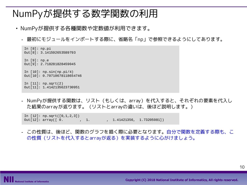
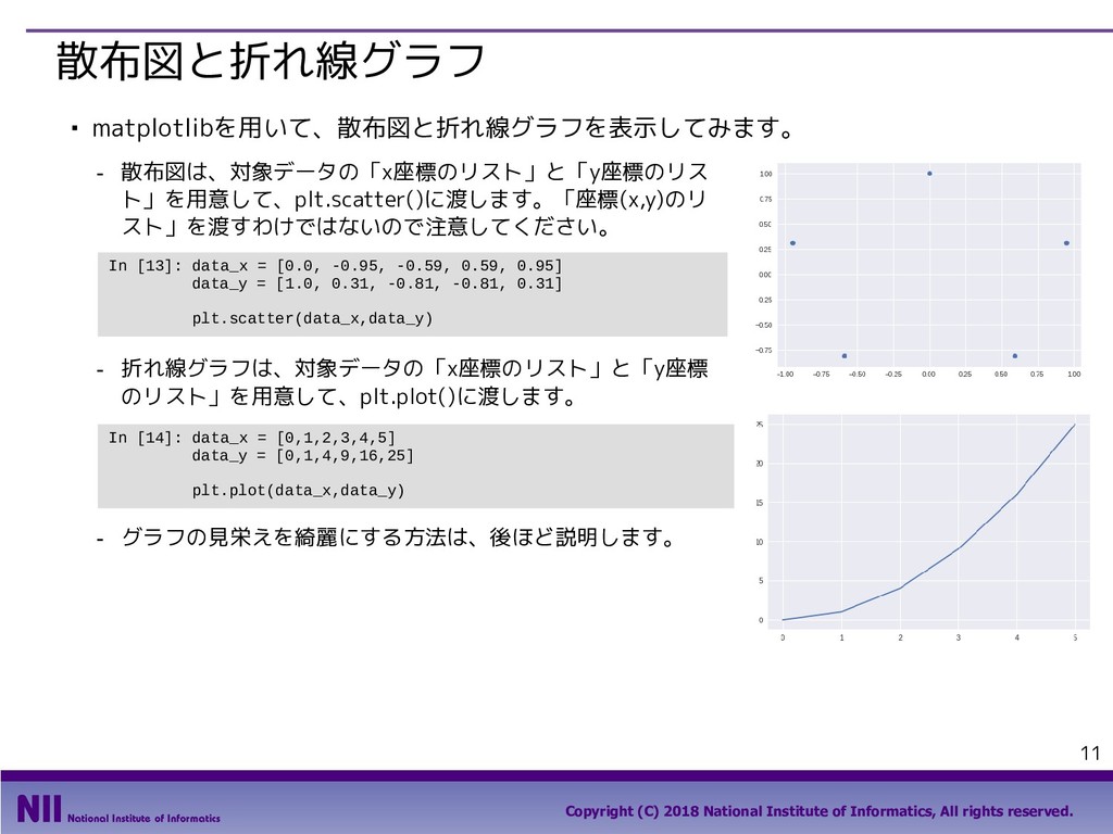
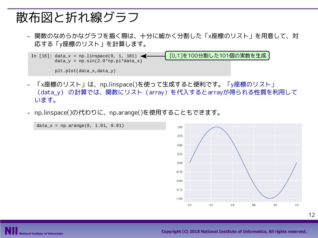
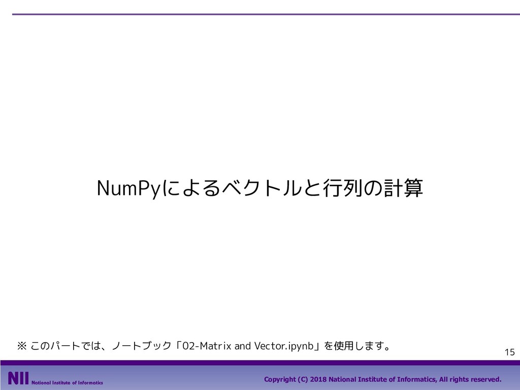
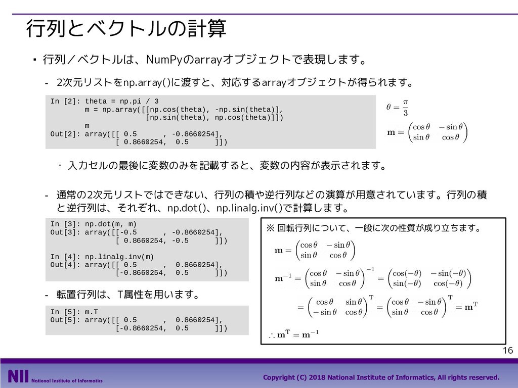
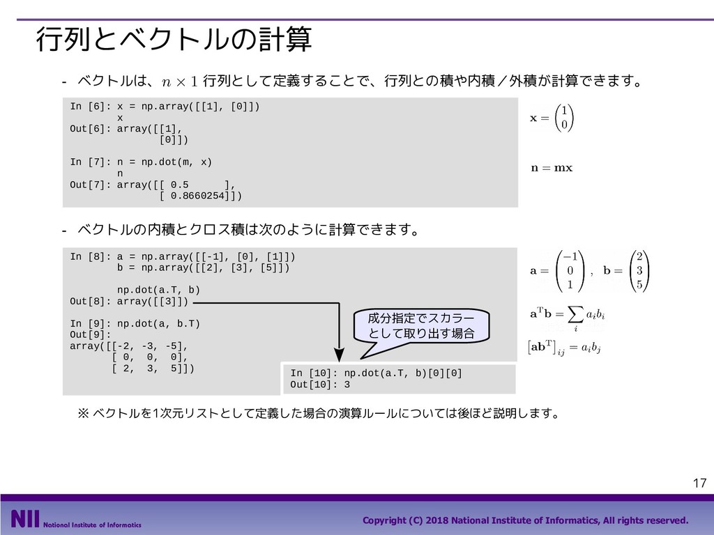
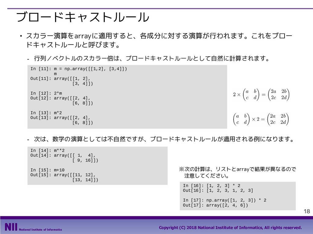
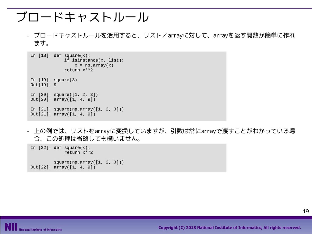
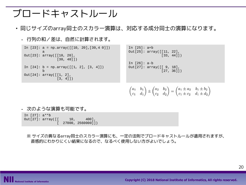
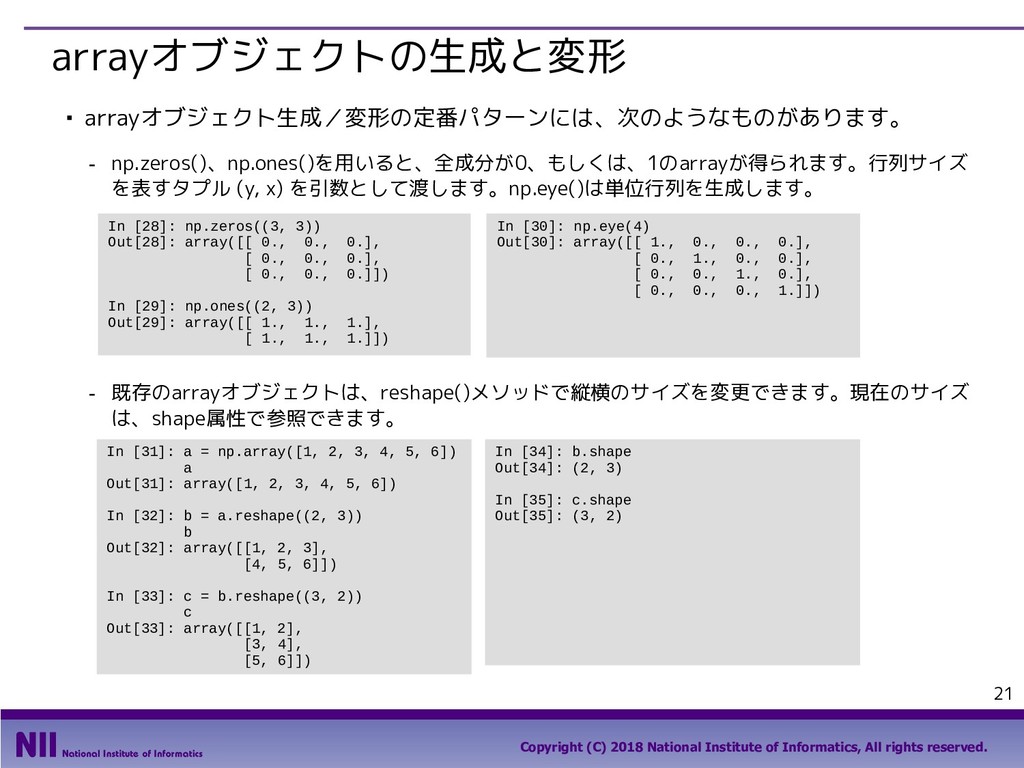
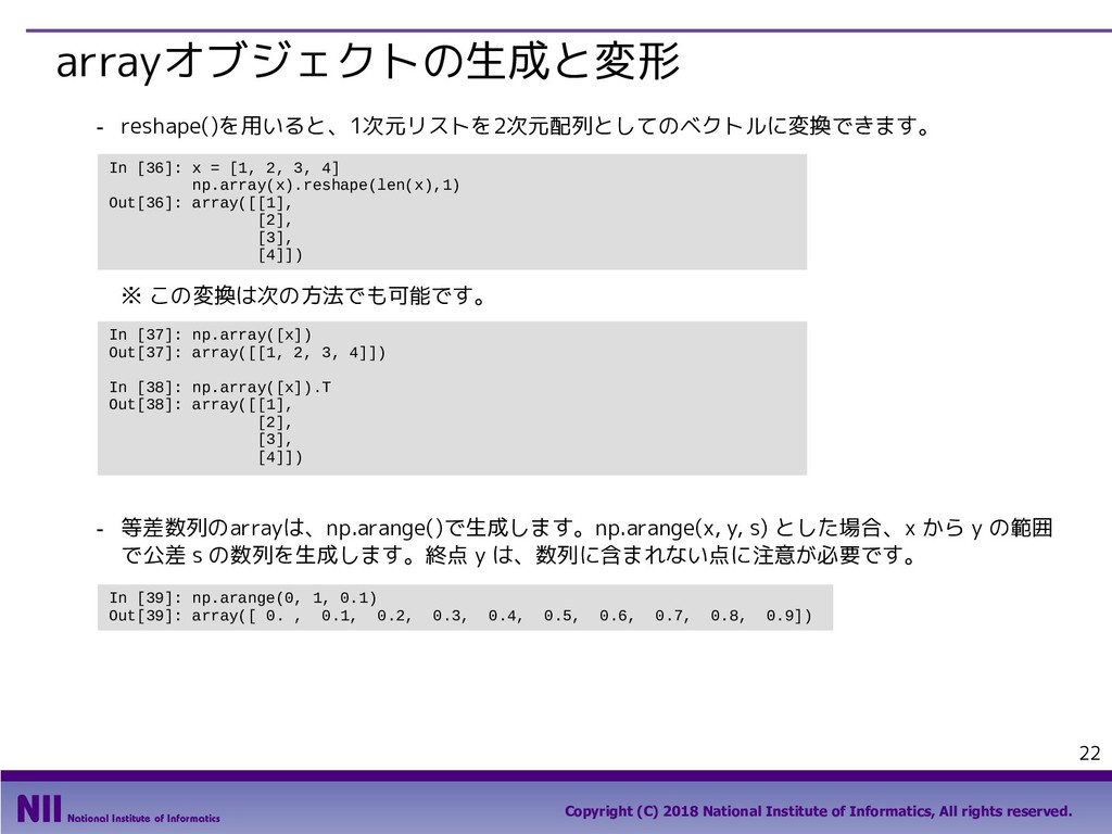
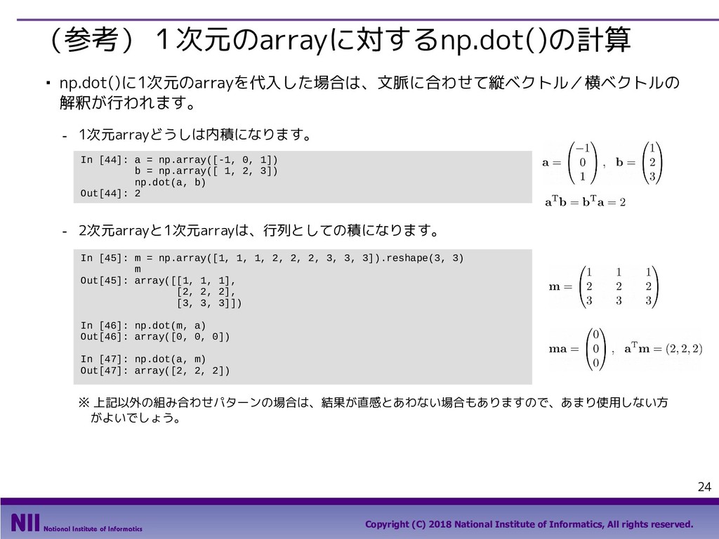
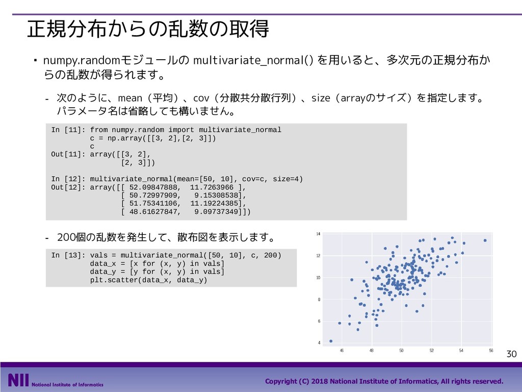
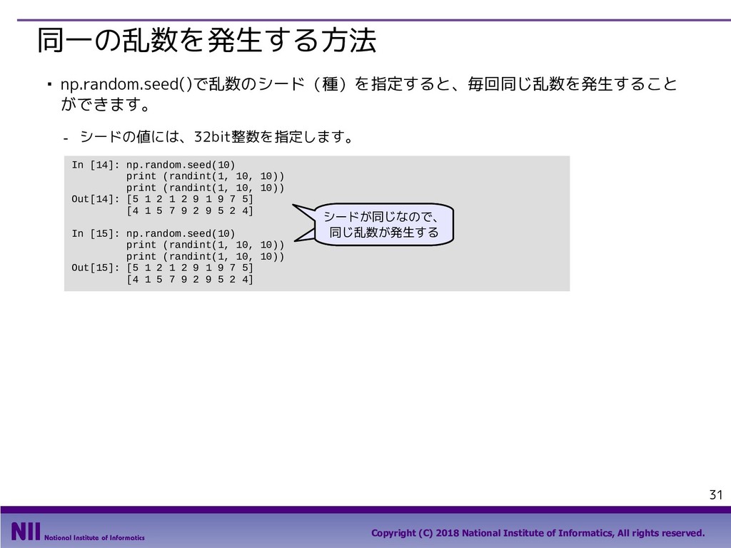
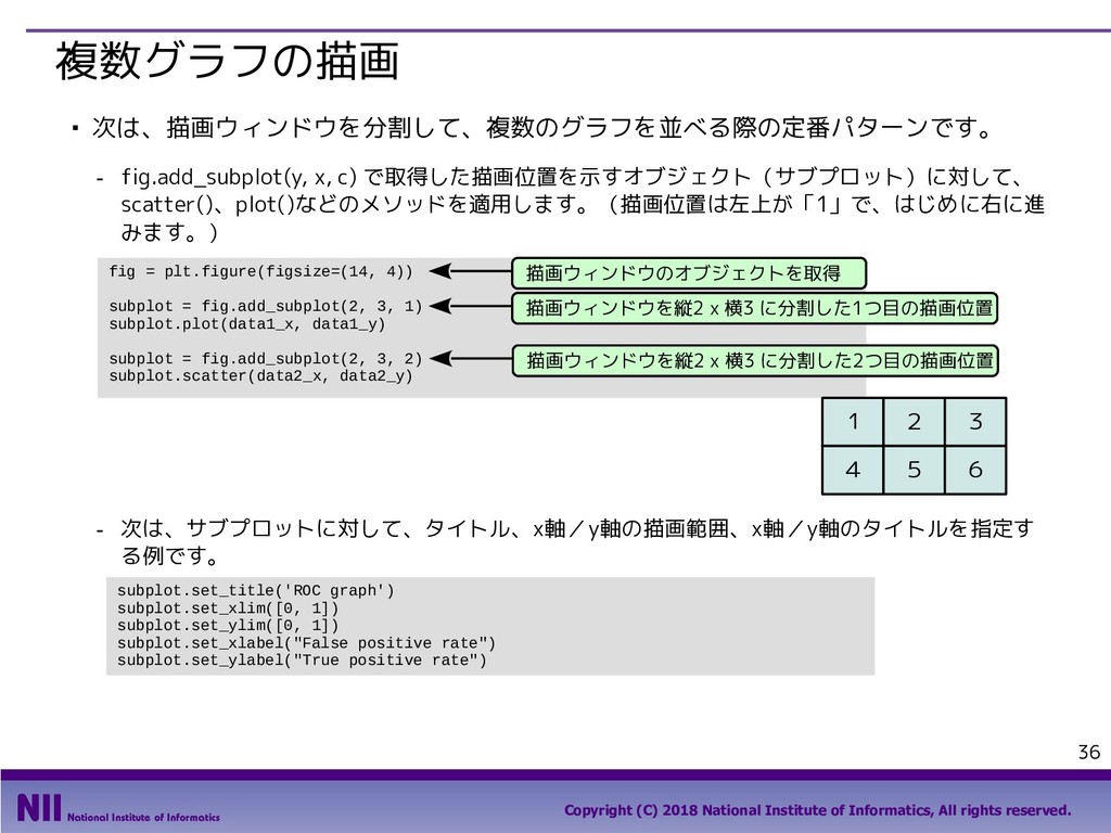
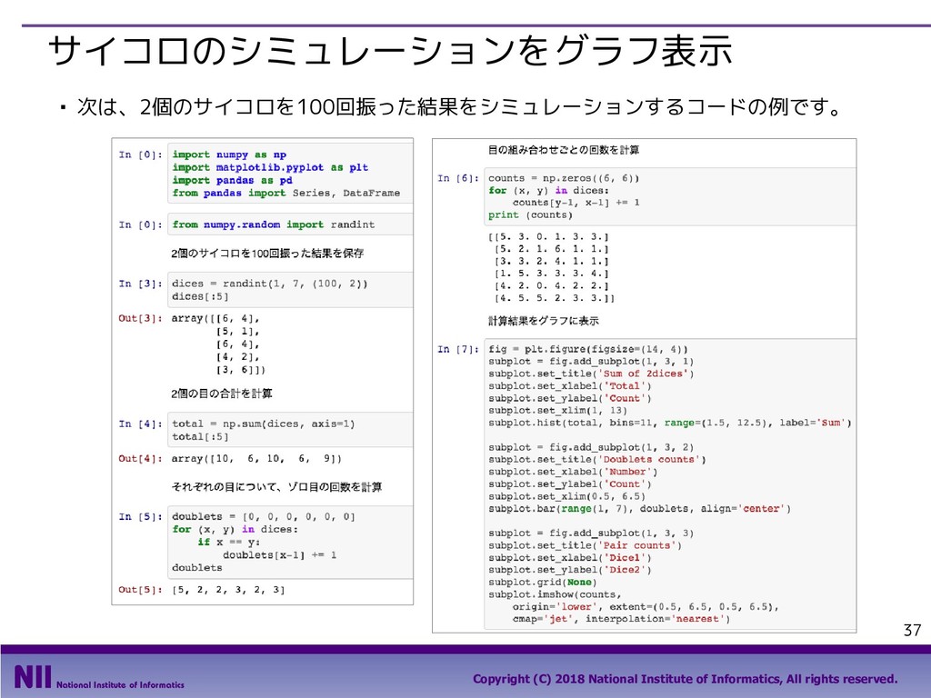
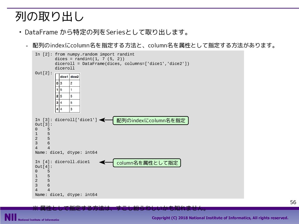
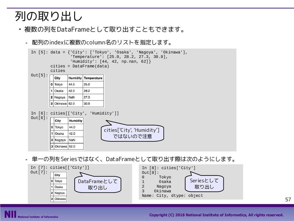
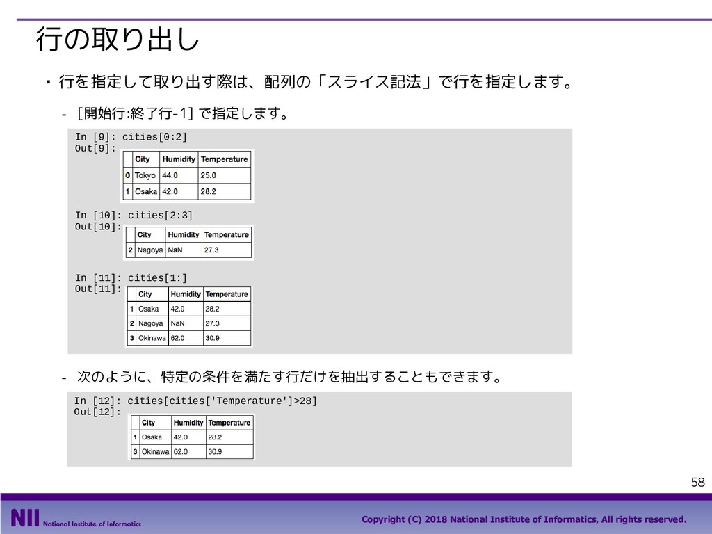
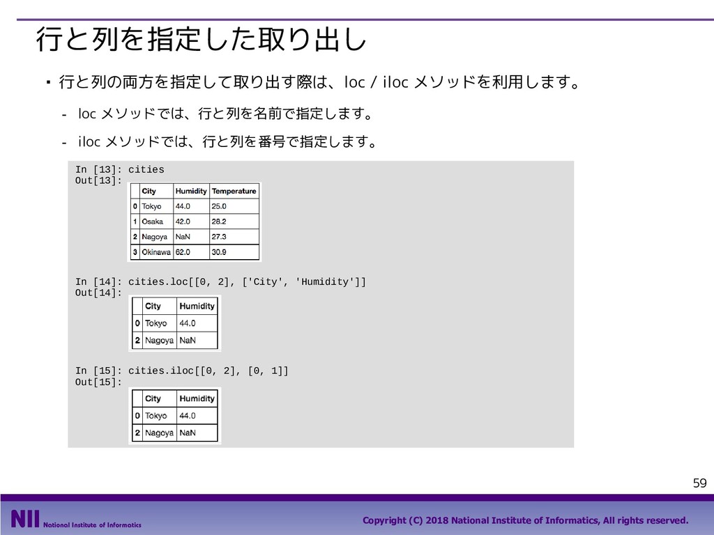
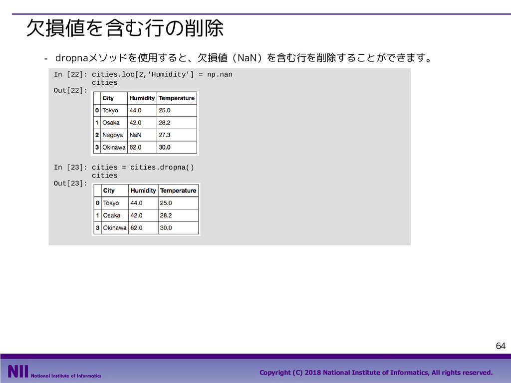
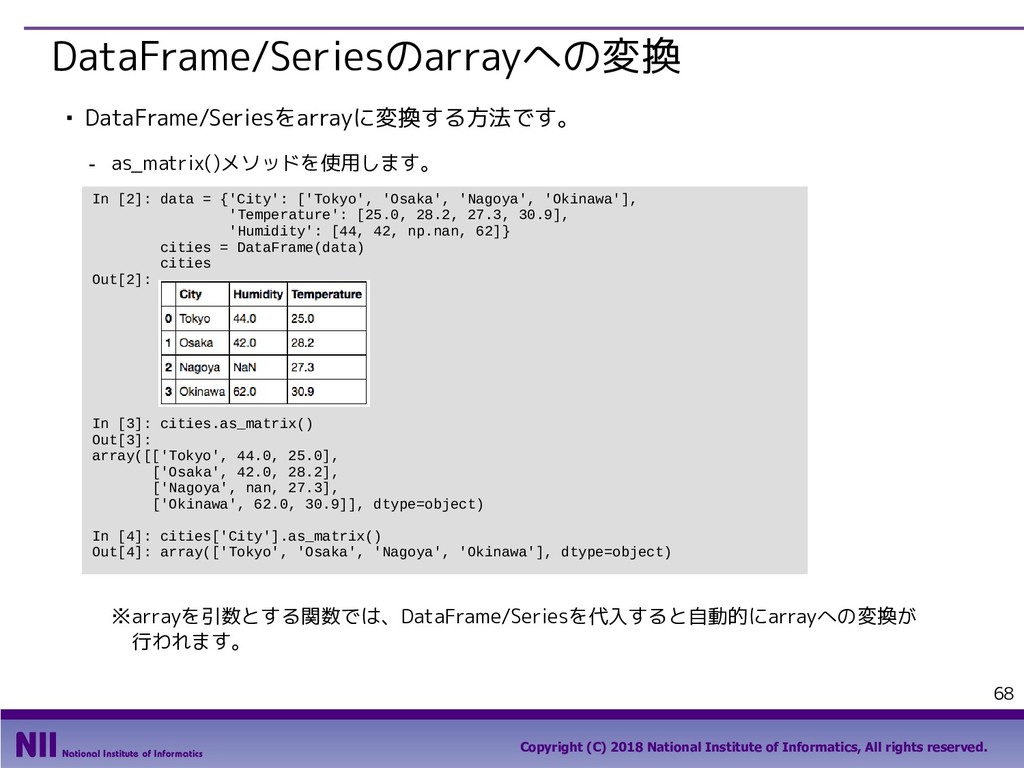
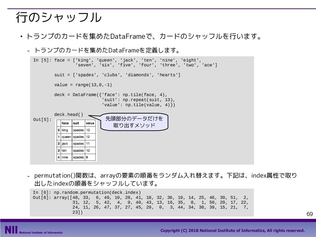
All rights reserved. 69 行のシャッフル ▪ トランプのカードを集めたDataFrameで、カードのシャッフルを行います。 - トランプのカードを集めたDataFrameを定義します。 - permutation()関数は、arrayの要素の順番をランダム入れ替えます。下記は、index属性で取り出したindexの順番をシャッフルしています。 In [5]: face = ['king', 'queen', 'jack', 'ten', 'nine', 'eight', 'seven', 'six', 'five', 'four', 'three', 'two', 'ace'] suit = ['spades', 'clubs', 'diamonds', 'hearts'] value = range(13,0,-1) deck = DataFrame({'face': np.tile(face, 4), 'suit': np.repeat(suit, 13), 'value': np.tile(value, 4)}) deck.head() Out[5]: In [6]: np.random.permutation(deck.index) Out[6]: array([48, 33, 6, 49, 10, 28, 41, 18, 32, 36, 19, 14, 25, 46, 30, 51, 2, 31, 12, 5, 42, 4, 9, 40, 43, 13, 16, 35, 8, 1, 50, 20, 17, 22, 24, 11, 26, 47, 37, 27, 45, 29, 0, 3, 44, 34, 38, 39, 15, 21, 7, 23]) 先頭部分のデータだけを取り出すメソッド

All rights reserved. 70 行のシャッフル - reindex()メソッドは、DataFrameのindexを付け直します。先のシャッフルしたindexを与えることで、行のシャッフルを行います。 - さらに、reset_index()でindexに通し番号を付け直すこともできます。 ※ 「drop=True」を指定しない場合、古いindexが「index」というcolumnに保存されます。 In [7]: deck = deck.reindex(np.random.permutation(deck.index)) deck.head() Out[7]: In [8]: deck = deck.reset_index(drop=True) deck.head() Out[8]:

All rights reserved. 71 In [9]: result = DataFrame() for c in range(3): y = 0 t = [] for delta in np.random.normal(loc=0.0, scale=1.0, size=100): y += delta t.append(y) result['Trial %d' % c] = t result.head() Out[9]: In [10]: result.plot(title='Random walk') データフレームによるグラフの描画 ▪ DataFrameオブジェクトは自分自身のグラフを描く機能を持っています。 - 次のようにplot()メソッドを用いると、列ごとのデータをまとめてグラフに表示することができます。 ※ plot()メソッドの詳細は下記を参照　http://pandas.pydata.org/pandas-docs/version/0.17.0/visualization.html

All rights reserved. 77 In [2]: def create_dataset(num): dataset = DataFrame(columns=['x', 'y']) for i in range(num): x = float(i)/float(num-1) y = np.sin(2*np.pi*x) + normal(scale=0.3) dataset = dataset.append(Series([x,y], index=['x', 'y']), ignore_index=True) return dataset In [3]: train_set = create_dataset(10) In [4]: train_set In [5]: train_set.plot(kind='scatter', x='x', y='y', xlim=[-0.1,1.1], ylim=[-1.5,1.5]) サンプルデータの作成 ▪ 区間　　　　　を等分したデータセットを生成します。 - (x, y) 座標を列に持つDataFrameとして用意します。ここでは、空のデータフレームに、1行ずつSeriesオブジェクトを追加する方法で作成しています。

All rights reserved. 78 サンプルデータの作成 - NumPyの機能を活用して、arrayオブジェクトをDataFrameに変換する方法を用いると、もっとシンプルに実装することも可能です。 In [6]: def create_dataset(num): data_x = np.linspace(0, 1, num) data_y = np.sin(2*np.pi*data_x) + normal(loc=0, scale=0.3, size=num) dataset = DataFrame({'x': data_x, 'y': data_y}) return dataset

All rights reserved. 79 係数の決定 ▪ 最小二乗法の公式を用いて、多項式の係数を計算します。 - 次の関数では、決定された多項式　　と係数　を返しています。 In[7] : def resolve(dataset, m): t = dataset.y phi = DataFrame() for i in range(0, m+1): p = dataset.x**i p.name="x**%d" % i phi = pd.concat([phi, p], axis=1) tmp = np.linalg.inv(np.dot(phi.T, phi)) ws = np.dot(np.dot(tmp, phi.T), t) def f(x): y = 0 for i, w in enumerate(ws): y += w * (x ** i) return y return (f, ws)

All rights reserved. 80 係数の決定 - 各変数の内容を表示すると、次のようになります。 - 行列　は、DataFrameに列を追加する方法で作成しています。 In[8] : def resolve(dataset, m): t = dataset.y print ("\nt:") print (t) phi = DataFrame() for i in range(0,m+1): p = dataset.x**i p.name="x**%d" % i phi = pd.concat([phi,p], axis=1) print ("\nphi:") print (phi) tmp = np.linalg.inv(np.dot(phi.T, phi)) ws = np.dot(np.dot(tmp, phi.T), t) print ("\nws:") print (ws) def f(x): y = 0 for i, w in enumerate(ws): y += w * (x ** i) return y return (f, ws) In[9] : f = resolve_debug(train_set, 3) t: 0 -0.176290 1 0.406402 2 0.592576 3 1.175387 4 0.652480 5 -0.477052 6 -1.123978 7 -0.720408 8 -0.417265 9 -0.253635 Name: y, dtype: float64 phi: x**0 x**1 x**2 x**3 0 1 0.000000 0.000000 0.000000 1 1 0.111111 0.012346 0.001372 2 1 0.222222 0.049383 0.010974 3 1 0.333333 0.111111 0.037037 4 1 0.444444 0.197531 0.087791 5 1 0.555556 0.308642 0.171468 6 1 0.666667 0.444444 0.296296 7 1 0.777778 0.604938 0.470508 8 1 0.888889 0.790123 0.702332 9 1 1.000000 1.000000 1.000000 ws: [ -0.29207698, 11.0815224 , -30.56215955, 19.6937635 ]

All rights reserved. 81 平方根平均二乗誤差の計算 ▪ 決定された多項式を用いて、平方根平均二乗誤差を計算します。 - 次はiterrows()メソッドで、データセット dataset の各要素についての繰り返し処理を行っています。 - NumPyのブロードキャストルールを利用すると、次のように1行で計算することも可能です。 In [10]: def rms_error(dataset, f): err = 0 for index, line in dataset.iterrows(): x, y = line.x, line.y err += 0.5 * (y - f(x))**2 return np.sqrt(2 * err / len(dataset)) In [11]: def rms_error(dataset, f): return np.sqrt(np.sum((dataset.y - f(dataset.x))**2)/len(dataset))

All rights reserved. 82 In [12]: def show_result(subplot, train_set, m): f = resolve(train_set, m) subplot.set_xlim(-0.05, 1.05) subplot.set_ylim(-1.5, 1.5) subplot.set_title("M=%d" % m) # トレーニングセットを表示 subplot.scatter(train_set.x, train_set.y, marker='o', color='blue', label=None) # 真の曲線を表示 linex = np.linspace(0, 1, 101) liney = np.sin(2*np.pi*linex) subplot.plot(linex, liney, color='green', linestyle='--') # 多項式近似の曲線を表示 linex = np.linspace(0, 1, 101) liney = f(linex) label = "E(RMS)=%.2f" % rms_error(train_set, f) subplot.plot(linex, liney, color='red', label=label) subplot.legend(loc=1) In [13]: fig = plt.figure(figsize=(8, 6)) for i, m in enumerate([0, 1, 3, 9]): subplot = fig.add_subplot(2, 2, i+1) show_result(subplot, train_set, m) 分析結果のグラフ表示 ▪ 決定された多項式の曲線など、分析結果をまとめてグラフに表示します。 - subplotオブジェクトを受け取って、その部分にグラフを描く関数を用意します。 - 次は、4種類のグラフをまとめて描きます。

All rights reserved. 83 平方根平均二乗誤差の変化 ▪ 多項式の次数にともなう平方根平均二乗誤差の変化を計算します。 - 次はトレーニングセットとテストセットについて、それぞれの平方根平均二乗誤差を計算しています。　　　　の各次数での結果をDataFrameにまとめて、グラフを表示します。 In [14]: def show_rms_trend(train_set, test_set): df = DataFrame(columns=['Training set', 'Test set']) for m in range(0, 10): # 多項式の次数 f = resolve(train_set, m) train_error = rms_error(train_set, f) test_error = rms_error(test_set, f) df = df.append(Series([train_error, test_error], index=['Training set', 'Test set']), ignore_index=True) df.plot(title='RMS Error', style=['-', '--'], grid=True, ylim=(0, 0.9))

All rights reserved. 84 In [15]: def show_rms_trend(train_set, test_set): df = DataFrame(columns=['Training set','Test set']) for m in range(0,10): # 多項式の次数 f = resolve(train_set, m) train_error = rms_error(train_set, f) test_error = rms_error(test_set, f) df = df.append(Series([train_error, test_error], index=['Training set','Test set']), ignore_index=True) print (df) df.plot(title='RMS Error', style=['-','--'], grid=True, ylim=(0,0.9)) In [16]: train_set = create_dataset(10) test_set = create_dataset(10) show_rms_trend_debug(train_set, test_set) Training set Test set 0 0.654370 0.743018 1 0.465365 0.573458 2 0.462929 0.576735 3 0.138445 0.281417 4 0.136046 0.290995 5 0.126021 0.280504 6 0.071521 0.293895 7 0.013880 0.310773 8 0.013857 0.311028 9 0.000186 0.314195 平方根平均二乗誤差の変化 - 次は実際に平方根平均二乗誤差をまとめたDataFrameの例です。 DataFrameの機能でグラフを表示

All rights reserved. 89 サンプルデータの作成 ▪ 　　　の属性を持つデータセットを用意します。 - 次の関数では、(x, y, t) それぞれの値を列とするDataFrameにまとめています。 In[2] : def prepare_dataset(n1, mu1, variance1, n2, mu2, variance2): df1 = DataFrame(multivariate_normal(mu1, np.eye(2)*variance1 ,n1), columns=['x', 'y']) df1['type'] = 1 df2 = DataFrame(multivariate_normal(mu2, np.eye(2)*variance2, n2), columns=['x', 'y']) df2['type'] = -1 df = pd.concat([df1,df2], ignore_index=True) df = df.reindex(np.random.permutation(df.index)).reset_index(drop=True) return df In[3] : train_set = prepare_dataset(20, [15, 10], 15, 30, [0, 0], 15) In [4]: train_set.head(10)

All rights reserved. 90 サンプルデータの作成 ▪ 先の関数の処理の流れは、次のようになります。 - はじめに、　　　それぞれのデータを個別のDataFrameとして用意します。　 - np.random.multivariate_normal() で2次元正規分布のDataFrameを作成して、その後で、type の列を追加しています。 - ２つのDataFrameを結合して行をシャッフルすることで、最終的なデータセットとしています。 In [6]: train_set = prepare_dataset_debug(20, [15, 10], 15, 30, [0, 0], 15) df1: x y type 0 16.781857 13.639916 1 1 16.884073 6.919148 1 2 12.056751 4.794741 1 3 12.730577 14.388435 1 4 11.577948 9.154710 1 df2: x y type 0 1.323629 2.003764 -1 1 1.874265 2.324382 -1 2 1.760324 1.896797 -1 3 -2.279221 -2.780630 -1 4 -3.115091 5.504012 -1 In[5] : def prepare_dataset_debug(n1, mu1, variance1, n2, mu2, variance2): df1 = DataFrame(multivariate_normal(mu1, np.eye(2)*variance1 ,n1), columns=['x','y']) df1['type'] = 1 print ('\ndf1:') print (df1.head()) df2 = DataFrame(multivariate_normal(mu2, np.eye(2)*variance2, n2), columns=['x','y']) df2['type'] = -1 print ('\ndf2:') print (df2.head()) df = pd.concat([df1,df2], ignore_index=True) df = df.reindex(np.random.permutation(df.index)).reset_index(drop=True) return df df = pd.concat([df1, df2], ignore_index=True) df = df.reindex(np.random.permutation(df.index)).reset_index(drop=True) return df

All rights reserved. 91 パーセプトロンによる係数の決定 ▪ 次はパーセプトロンのアルゴリズムで係数を修正する処理の流れです。 - iterrows()メソッドでトレーニングセットの各データについて、「正しく分類されない点について係数の修正を行う」という処理を行ないます。この処理を30回繰り返して、それぞれの回を終えた時点の係数をDataFrameとして記録していきます。　　　 In [7] : def run_train(train_set): # パラメータの初期値とbias項の設定 w0 = w1 = w2 = 0.0 bias = 0.5 * (train_set.x.abs().mean() + train_set.y.abs().mean()) # Iterationを実施 paramhist = DataFrame([[w0, w1, w2]], columns=['w0', 'w1', 'w2']) for i in range(30): for index, point in train_set.iterrows(): x, y, type = point.x, point.y, point.type if type * (w0*bias + w1*x + w2*y) <= 0: w0 += type * bias w1 += type * x w2 += type * y paramhist = paramhist.append(Series([w0, w1 w2], ['w0', 'w1', 'w2']), ignore_index=True) # 判定誤差の計算 err = 0 for index, point in train_set.iterrows(): x, y, type = point.x, point.y, point.type if type * (w0*bias + w1*x + w2*y) <= 0: err += 1 err_rate = err * 100 / len(train_set) return paramhist, err_rate 正しく分類されない点について係数を修正

All rights reserved. 92 In [8]: paramhist, err_rate = run_train(train_set) paramhist.head(10) In [9]: paramhist.plot.legend(loc=1) パーセプトロンによる係数の決定 - 係数の変化を記録したDataFrameの様子です。DataFrameの機能を利用して、グラフを描くことができます。

All rights reserved. 93 グラフの描画 ▪ トレーニングセットのデータと決定された直線は、サブプロットオブジェクトの scatter()、および、plot()メソッドで表示しています。 In [10]: def show_result(subplot, train_set, w0, w1, w2, err_rate): train_set1 = train_set[train_set['type']==1] train_set2 = train_set[train_set['type']==-1] bias = 0.5 * (train_set.x.mean() + train_set.y.mean()) ymin, ymax = train_set.y.min()-5, train_set.y.max()+10 xmin, xmax = train_set.x.min()-5, train_set.x.max()+10 subplot.set_ylim([ymin-1, ymax+1]) subplot.set_xlim([xmin-1, xmax+1]) subplot.scatter(train_set1.x, train_set1.y, marker='o', label=None) subplot.scatter(train_set2.x, train_set2.y, marker='x', label=None) linex = np.arange(xmin-5, xmax+5) liney = - linex * w1 / w2 - bias * w0 / w2 label = "ERR %.2f%%" % err_rate subplot.plot(linex, liney, label=label, color='red') subplot.legend(loc=1) In [11] : fig = plt.figure() subplot = fig.add_subplot(1, 1, 1) params = paramhist[-1:] w0, w1, w2 = float(params.w0), float(params.w1), float(params.w2) show_result(subplot, train_set, w0, w1, w2, err_rate) t=±1のデータを個別に取り出し一番最後の係数の値を取り出し

All rights reserved. 96 参考資料 ▪ 『Pythonによるデータ分析入門 ―― NumPy、pandasを使ったデータ処理』 Wes McKinney（著）、小林儀匡、鈴木宏尚、瀬戸山雅人、滝口開資、野上大介（翻訳）、オライリージャパン（2013） - NumPyやpandasなど、データ解析に使用する標準的なPythonライブラリの使用方法を解説しています。 ▪ 『Think Stats 第2版 ―プログラマのための統計入門』 Allen B. Downey（著）、黒川利明（翻訳）、黒川洋（翻訳）、オライリージャパン（2015） - 統計解析の実例をPythonで実装しながら解説しています。

Data Analysis Libraries

Data Analysis Libraries

More Decks by Etsuji Nakai

Other Decks in Technology

Featured

Transcript