Analyst’s Nightmare or Laundering Massive Spreadsheets

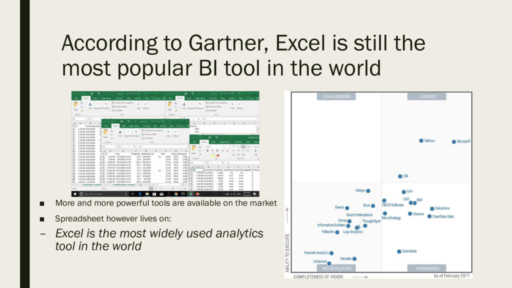
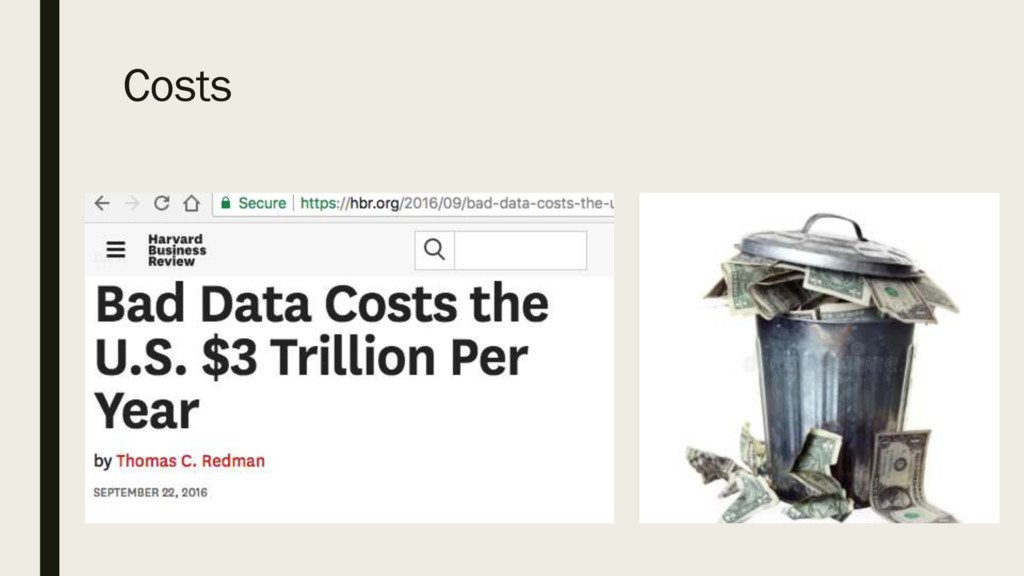
The spreadsheet lives on, especially in sectors slow to adopt new technology, such as medicine and  nance. Not only data is frequently stored and passed around in the
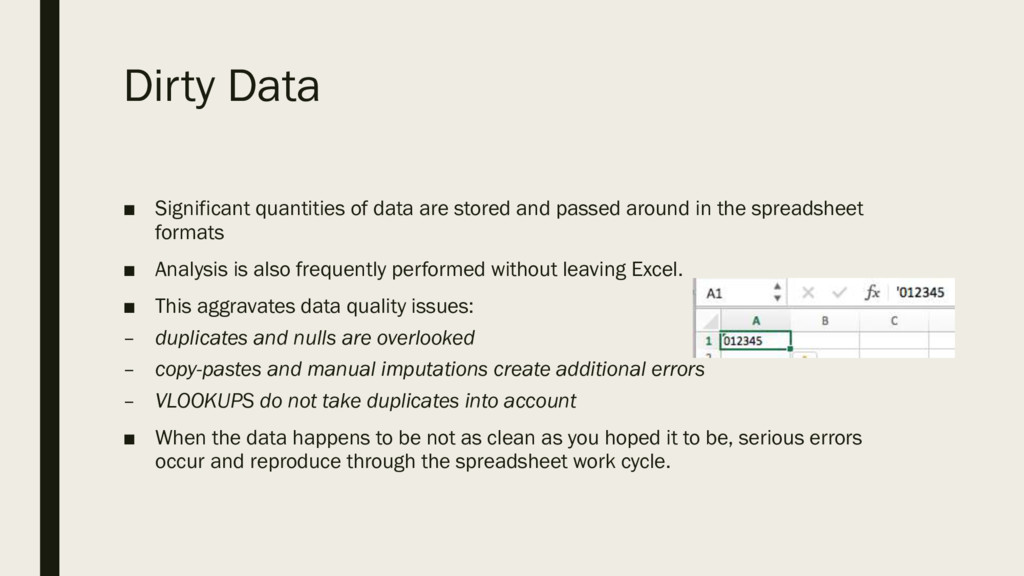
spreadsheet formats, analysis is also frequently performed without leaving Excel. And when the data happens to be not as clean as you hoped it to be, serious errors occur and
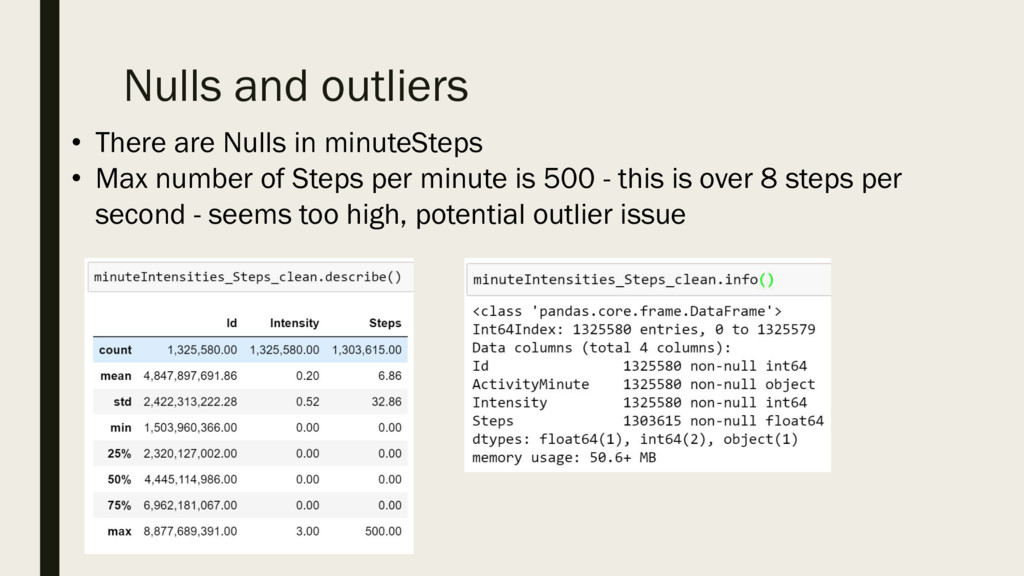
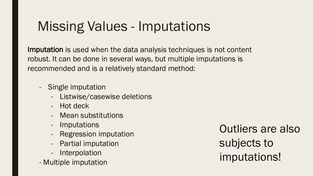
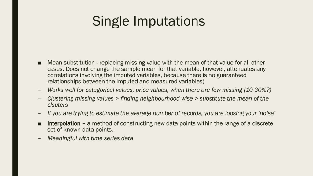
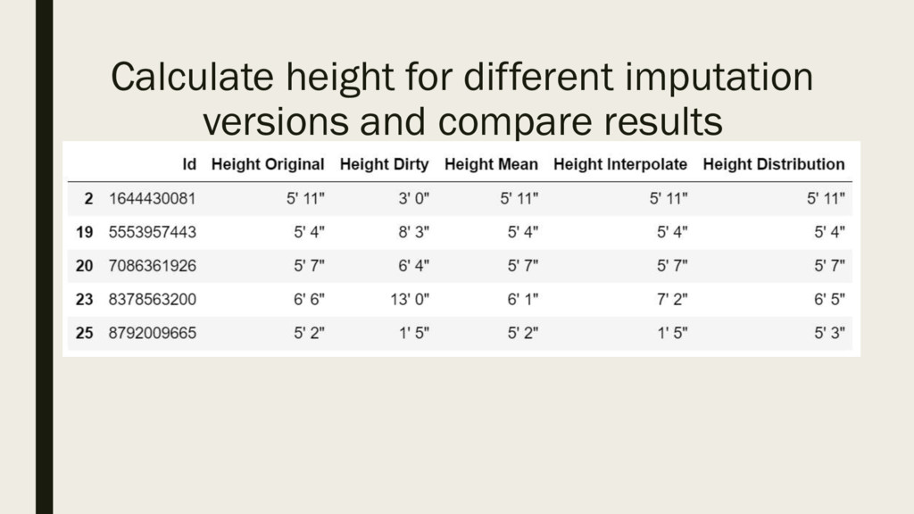
reproduce through the spreadsheet workcycle. Data quality issues such as duplicates and nulls, common practices such as copy-pastes, VLOOKUPS, and manual imputations as
well as failure to properly understand and clean the data prior to making conclusions frequently lead to signi cant errors.
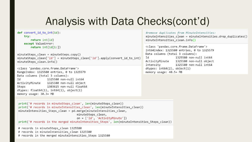
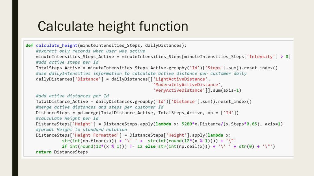
Pandas library provides a powerful tool of ingesting, cleaning, transforming, and visualizing spreadsheet data that are either lacking in Excel or are very painful to implement
given the number of worksheets required for a task. This talk will demonstrate several frequently occurring data issues and show how they can be dealt with in Pandas. We will
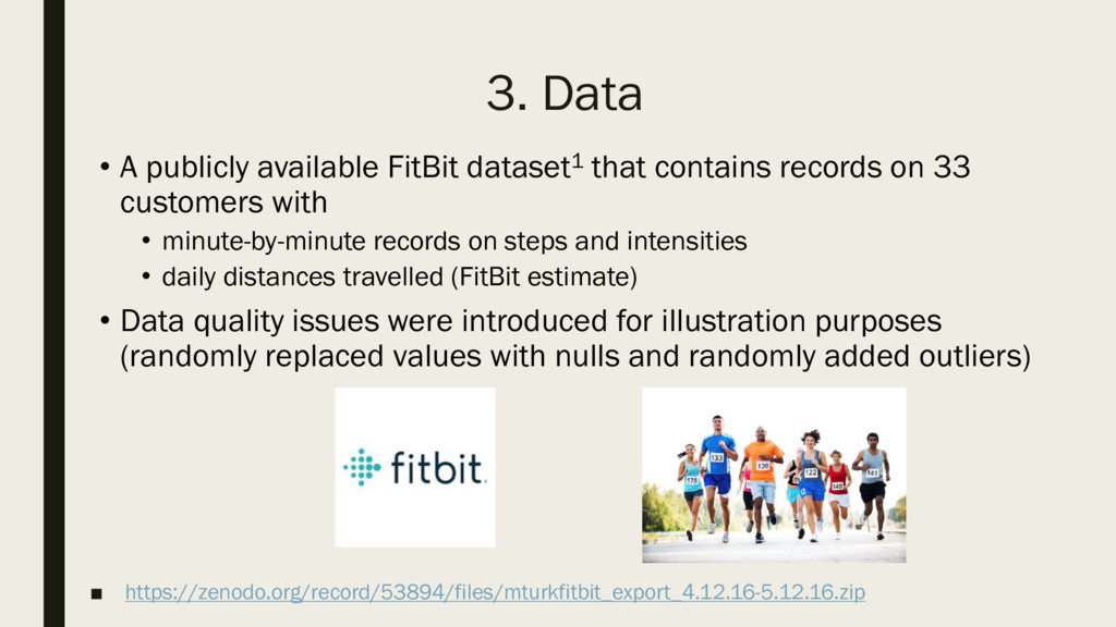
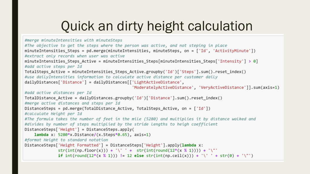
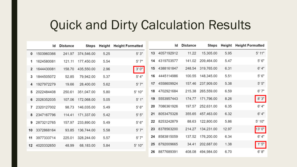
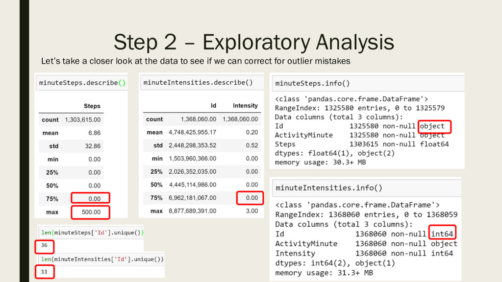
start with an example of an analysis performed in an Excel spreadsheet and will perform step by step invalidation of its conclusions. For this talk we will use a synthetic dataset
that artificially combines multiple data issues encountered in real life and provides a good illustration of common data pitfalls.
Co-presented with Tanya Yarmola

Transcript

1. ANALYST’S NIGHTMARE OR LAUNDERING MASSIVE SPREADSHEETS An example of how analysis that overlooks data quality issues may go completely wrong By Feyzi Bagirov and Tanya Yarmola
2. Agenda ▪ About us ▪ Excel is The King ▪ Dirty Data ▪ FitBit dataset intro – Fit Bit dataset insights (pre-impute) – Fit Bit dataset insights (post-impute) ▪ Q&A
3. About us ▪ Vice President in Model Governance and Review at JP Morgan ▪ Faculty of Analytics at Harrisburg University of Science and Technology ▪ Data Science Advisor at Metadata.io
4. 1. Excel is The King
5. Use Case: implementation of a new BI tool in 2007 – present day
6. According to Gartner, Excel is still the most popular BI tool in the world ▪ More and more powerful tools are available on the market ▪ Spreadsheet however lives on: – Excel is the most widely used analytics tool in the world
8. 2. Dirty Data
9. Dirty Data ▪ Significant quantities of data are stored and passed around in the spreadsheet formats ▪ Analysis is also frequently performed without leaving Excel. ▪ This aggravates data quality issues: – duplicates and nulls are overlooked – copy-pastes and manual imputations create additional errors – VLOOKUPS do not take duplicates into account ▪ When the data happens to be not as clean as you hoped it to be, serious errors occur and reproduce through the spreadsheet work cycle.
10. According to IDG, cleaning and organizing data takes up to 60% of the data scientists’ time
11. Costs
12. Bias Danger • Some members of the intended population are less likely to be included than others. • Results in a non-random sample of a population • Results can be erroneously attributed to the phenomenon under study rather than to the method of sampling.
13. Common types of dirty data ▪ Missing data – Missing Completely At Random (MCAR) – Missing At Random (MAR) – Missing Not At Random (MNAR) ▪ Duplicates ▪ Outliers ▪ Multiple comma-separated (or not) values that are stored in one column (common symptom) * ▪ Column headers are values, not variable names ▪ Encoding ** *. Pandas has a function called df.apply(), which will let you apply to every row or a column ** Pandas are Unicode sandwich compliant - the idea is the strings coming in should be decoded at the boundary of what you are doing, and then as they come out they should be encoded again.
14. Missing Completely At Random (MCAR) ▪ Data is MCAR if the events that lead to any particular data-item being missing are independent both of observable variables and of unobservable parameters of interest, and occur entirely at random ▪ Basically, data ”missingness” is unsystematic ▪ An example is when the survey data has not been completed because it was lost in the mail
15. Missing At Random (MAR) ▪ MAR occurs when the “missingness” is not random, but where “missingness” can be fully accounted for by variables where there is complete information ▪ An example, a depression survey is not filled out by men, not because they are not depressed, but because of the men ego.
16. Missing Not At Random (MNAR) ▪ When the data is neither MCAR nor MAR ▪ “Missingness” is specifically related to what is missing ▪ Example: a person does not attend a drug test, because he/she took the drugs the night before
17. Common causes of dirty data ▪ Mechanical errors ▪ Business rule violation ▪ Database mergers ▪ Data export and import
18. Concept of tidy data ▪ “Tidy Data” by Hadley Wickham, “Journal of Statistical Software”, Aug 20141 ▪ Principles of tidy data: – Observations as rows – Variables of columns – One type of observational unit per table (if table that suppose to contain characteristics of people, contains information about their pets, there are more observational units). 1 https://www.jstatsoft.org/article/view/v059i10/v59i10.pdf
19. General framework for data cleaning* Define and determine error types Search and identify error instances Correct the errors Document error instances and error types Modify data entry procedures to reduce future errors * Maletic & Marcus 2000
20. Handling Dirty Data ▪ "error prevention is far superior to error detection and cleaning, as it is cheaper and more efficient to prevent errors than to try and find them and correct them later” – Principles of Data Quality, Chapman
21. Handling Dirty Data ▪ You can handle dirty data on two levels: – Database level/manual clean inside the database – not efficient, does not scale well – Application level – recommended way, whenever possible Ø Identify the commonly occurring problems with your data and the tasks to fix them Ø Once you identified most common tasks related to your data cleanup, create scripts, that you are going to be run on every new dataset. Ø Whenever you have new type of errors in the new dataset, add the code to fix them to your scripts.
22. ▪ https://zenodo.org/record/53894/files/mturkfitbit_export_4.12.16-5.12.16.zip • A publicly available FitBit dataset1 that contains records on 33 customers with • minute-by-minute records on steps and intensities • daily distances travelled (FitBit estimate) • Data quality issues were introduced for illustration purposes (randomly replaced values with nulls and randomly added outliers) 3. Data
23. Objectives ▪ To provide a simple example that illustrates how data quality issues may visibly affect results of an analysis ▪ To estimate customer’s height based on average stride length and see whether results belong to expected ranges
24. Tools
25. Step 1 - Data Manipulations
26. Quick an dirty height calculation
27. Quick and Dirty Calculation Results
28. Step 2 – Exploratory Analysis Let’s take a closer look at the data to see if we can correct for outlier mistakes
29. Initial observations ▪ minuteSteps and minuteIntensities have different numbers of records - there may be duplicates. ▪ Most values for Steps and Intesities are zeroes. ▪ There are Nulls in minuteSteps ▪ Numbers of unique user Ids are different. ▪ Id in minuteSteps is an object datatype. ▪ Max number of Steps per minute is 500 - this is over 8 steps per second - seems too high, potential outlier issue
30. Daily Distances observations More observations • Number of unique Ids matches minuteIntensities • SedentaryActiveDistance is mostly zero – exclusion should be OK
31. Cleaning - Analysis with Data Checks • Ids are mix of integers and strange strings • Should convert all to integers to match other datasets
32. Analysis with Data Checks(cont’d)
33. Analysis with Data Checks(cont’d)
34. Nulls and outliers • There are Nulls in minuteSteps • Max number of Steps per minute is 500 - this is over 8 steps per second - seems too high, potential outlier issue
35. Missing Values - Imputations Imputation is used when the data analysis techniques is not content robust. It can be done in several ways, but multiple imputations is recommended and is a relatively standard method: - Single imputation - Listwise/casewise deletions - Hot deck - Mean substitutions - Imputations - Regression imputation - Partial imputation - Interpolation - Multiple imputation Outliers are also subjects to imputations!
36. Single Imputations ▪ Mean substitution - replacing missing value with the mean of that value for all other cases. Does not change the sample mean for that variable, however, attenuates any correlations involving the imputed variables, because there is no guaranteed relationships between the imputed and measured variables) – Works well for categorical values, price values, when there are few missing (10-30%?) – Clustering missing values > finding neighbourhood wise > substitute the mean of the clsuters – If you are trying to estimate the average number of records, you are loosing your ‘noise’ ▪ Interpolation – a method of constructing new data points within the range of a discrete set of known data points. – Meaningful with time series data
37. ▪ Partial deletion (Listwise deletion/casewise)- the most common means of dealing with missing data is listwise deletion (complete case), which is when all cases with missing values are deleted. If the data are MCAR, this will not add any bias, but it will decrease the power of the analysis (smaller sample size). ▪ Pairwise deletion – deleting a case when it is missing a variable required for a particular analysis, but including that case in analysis for which all required variables are present. The main advantage of this method is that it is straightforward and easy to implement. Single Imputations (cont’d) These methods are appropriate, as long as you don’t throw away too much data, and you still have enough data after the deletion
38. ▪ Hot-deck – a missing value is imputed from a randomly selected similar record. ▪ Cold deck – same as Hot-deck, but uses values from another dataset. ▪ Regression imputation - Available information for complete and incomplete cases is used to predict whether a value on a specific variable is missing or not. Fitted values from the regression model are then used to impute the missing values. It has the opposite problem of mean imputation – imputed data do not have an error term included in their estimation, thus the estimates fit perfectly along the regression line without any residual variance, causing relationships to be over identified and suggest greater precision in the imputed values, supplying no uncertainty about that value. – Be careful, because you are replacing an average per category, and might be loosing the “noise” Single Imputations (cont’d)
39. Multiple Imputations ▪ Multiple Imputation developed to deal with the problem of increased noise due to imputation by Rubin (1987). There are multiple methods of multiple imputation ▪ In these methods (with hot-deck or cold-deck), you are using multiple regression to randomly select different values and see how the result is changes ▪ Recommended when you don’t have enough data or you need to impute to many values ▪ The primary method is Multiple Imputation by Chained Equations (MICE) should be implemented only when the missing data follow the missing at random mechanism
40. Multiple Imputations (cont’d) ▪ Advantages of Multiple Imputation: – An advantage over single imputation is that MI is flexible and can be used in cases, where the data is MCAR, MAR, and even when the data is MNAR. – By imputing multiple times, multiple imputation certainly accounts for the uncertainty and range of values that the true value could have taken. – Not difficult to implement ▪ Disadvantages of Multiple Imputation: – Can be computationally expensive and not quite worth it. – Might not give you any additional benefits
41. Which methods are more reliable and when? • Mean substitution, for example, does not guarantee relationships between the imputed and measured values; • Hot Deck method has a risk of increased bias and false conclusions; • Single imputation does not take into account the uncertainty and treats the data as if the values are actual;
42. Steps distributions per intensity Single imputations - Impute nulls and outliers using different methods: 1. mean value (per user) 2. interpolate between existing values 3. draw from the distribution of existing values (per customer)
43. Single imputation - Impute using mean
44. Single imputation - impute using interpolation (replacing using the previous value) • There are multiple methods for interpolation(replace with average between the two, etc.), that can be specified in the interpolate()
45. Impute using transform with random choice (hot-deck) • We took the distribution of existing values for the steps and plugged it in. • transform() from pandas which transforms your data series into something else. • We the value was missing, we randomly drew it from another user
46. Calculate height function
47. Calculate height for different imputation versions and compare results
49. Takeaways • Fix data before you need it fixed - maintain data quality at the time the data is collected (drop down box vs type in data). • Cleaning data is important. Your model can be very sophisticated and valid, but if you feed it a dirty data, you will not get a meaningful outcome. • Use the proper types – saves you a lot of trouble over time. • Always ask why and investigate your nulls and outliers. • Data has a tendency to be used in unanticipated ways - think about what others will do to your data, re-usebility in terms of data • Documentation matters - document the dataset, where it came from, range of columns, how was this data gathered, etc.
50. Q&A
51. Thanks! Feyzi Bagirov, feyzi.bagirov@metadata.io, @FeyziBagirov Tanya Yarmola, tanya.yarmola@jpmorgan.com, @TanyaYarmola GitHub: https://github.com/fbagirov/FitBitDataCleanup