and High throughput In-memory storage, fast indexing, co-located ops, batch ops API and query language SQL-like against POJOs and schema-free documents. JDBC driver, lots of limitations ACID transactions Maintain full ACID compliance against your data set through full transaction semantics High availability and resiliency Fault tolerance through replication, cross-data center replication, auto-healing Data Tiering RAM and SSD
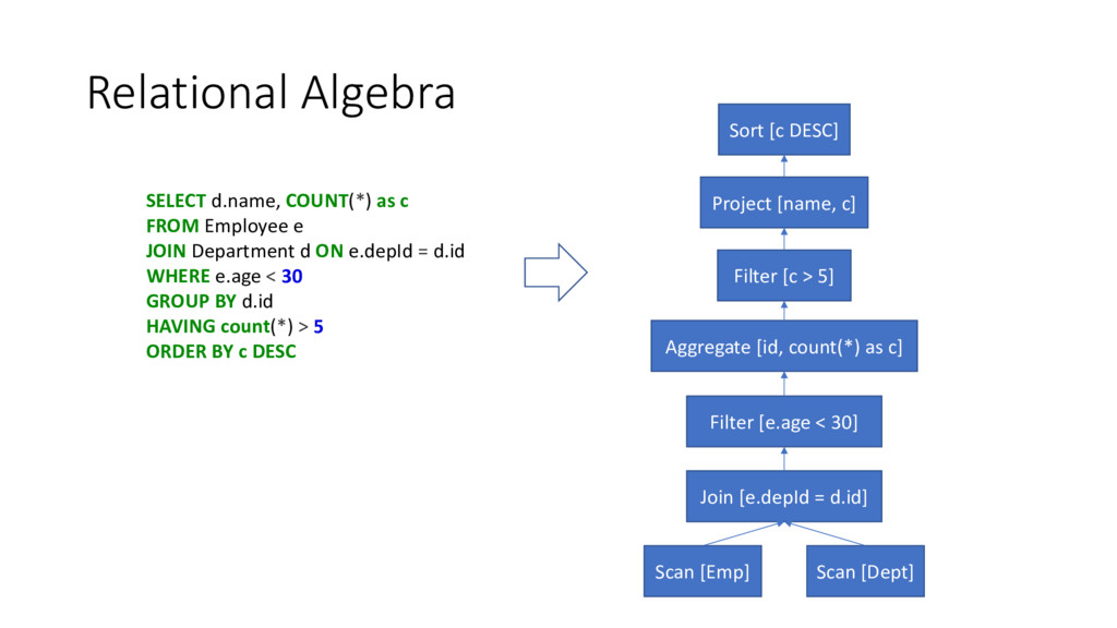
the options? • Enhance existing driver • custom SQL parser • extended SQL with ability to query embedded objects, geolocation • Create a new one • leverage industry-standard SQL parser, optimizer, JDBC driver • reimplement custom operations (though BI don’t support it) ”Modern relational query optimizers are complex pieces of code and typically represent 40 to 50 developer-years of effort” Raghu Ramakrishnan and Johannes Gehrke. Database Management Systems. Mc Graw Hill, 2000
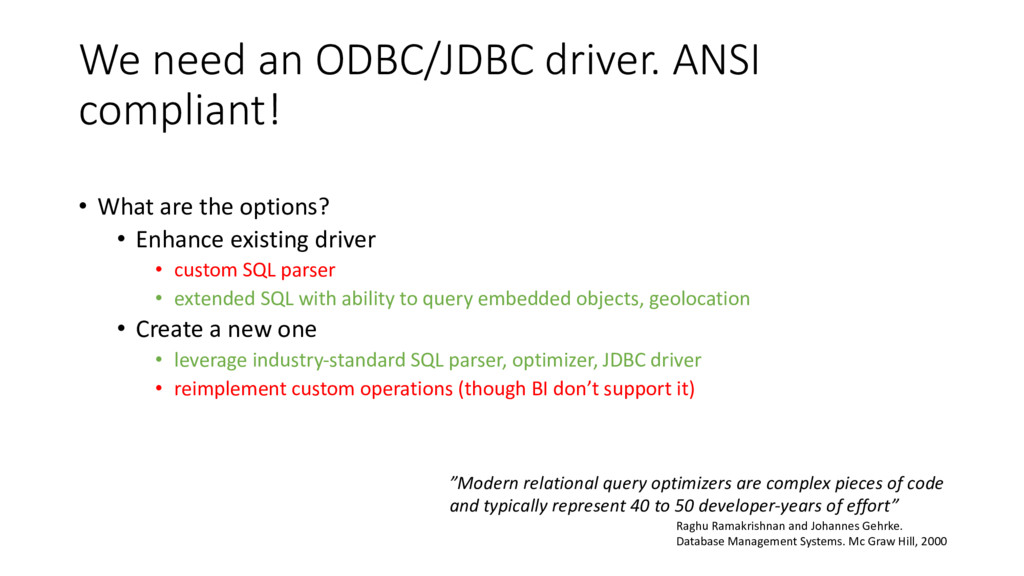
• Validate • validate against metadata • Optimize • logical plan is optimized and converted into physical expression • Execute • physical plan is converted into application-specific execution SQL Relational algebra Runnable query plan
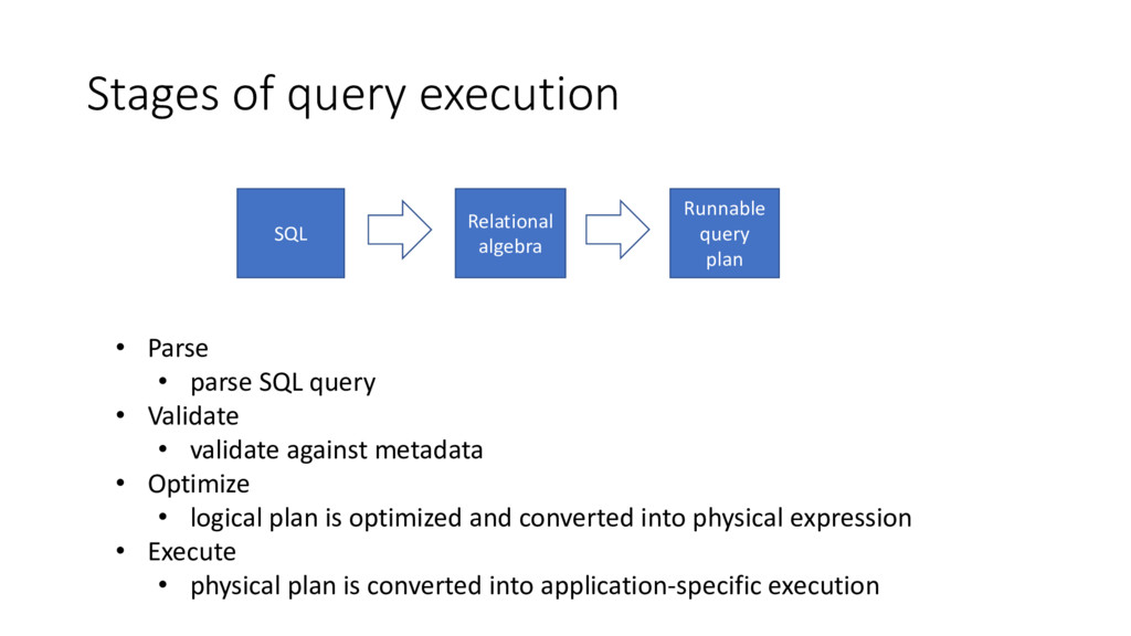
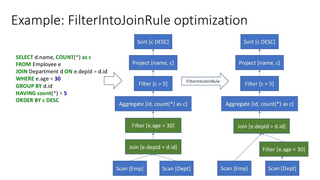
JOIN Department d ON e.depId = d.id WHERE e.age < 30 GROUP BY d.id HAVING count(*) > 5 ORDER BY c DESC Scan [Emp] Scan [Dept] Join [e.depId = d.id] Filter [e.age < 30] Aggregate [id, count(*) as c] Filter [c > 5] Project [name, c] Sort [c DESC]
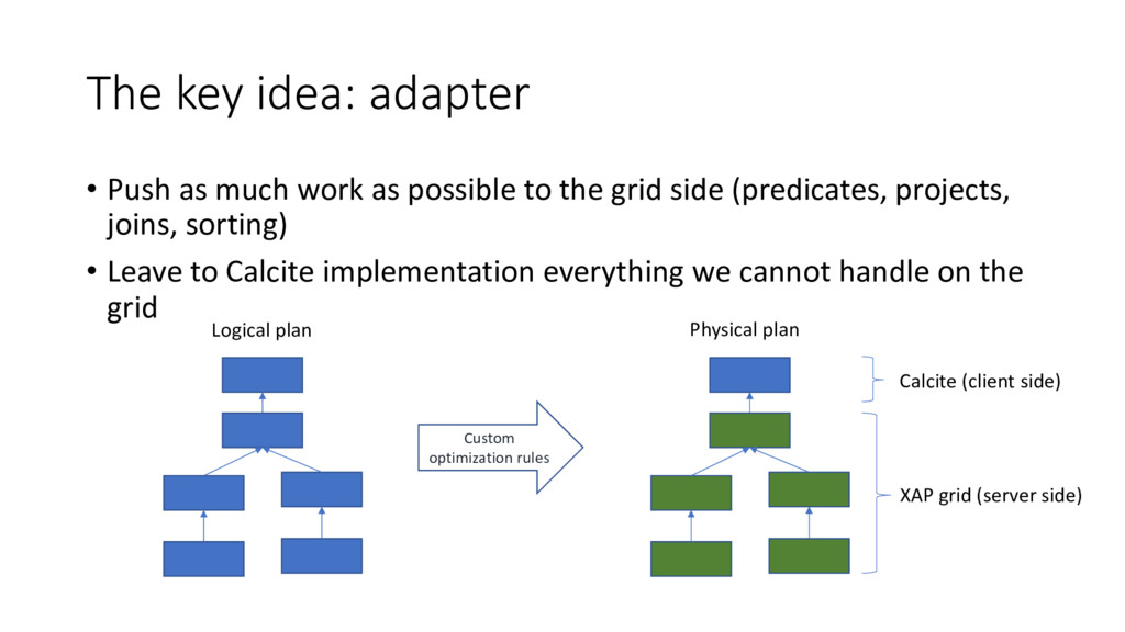
possible to the grid side (predicates, projects, joins, sorting) • Leave to Calcite implementation everything we cannot handle on the grid Custom optimization rules XAP grid (server side) Calcite (client side) Logical plan Physical plan
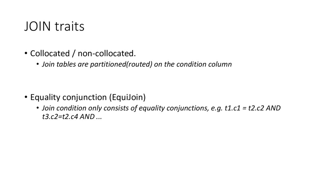
partitioned(routed) on the condition column • Equality conjunction (EquiJoin) • Join condition only consists of equality conjunctions, e.g. t1.c1 = t2.c2 AND t3.c2=t2.c4 AND ...
are partitioned(routed) on the condition column • All the data is available on a partition. • No data movement. • Distributed Task (kind-of MapReduce) • Join in mapper • Union record in reducer • Scales well Table A Table B Partition 2 Table A Table B Partition 3 Table A Table B
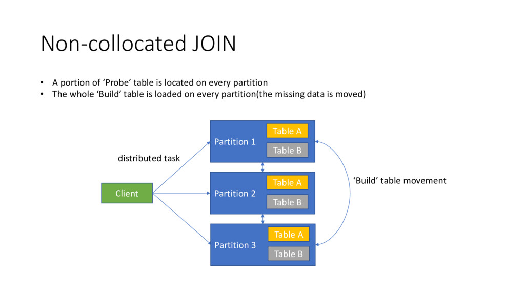
on every partition • The whole ‘Build’ table is loaded on every partition(the missing data is moved) Client Partition 1 distributed task Table A Table B Partition 2 Table A Table B Partition 3 Table A Table B ‘Build’ table movement
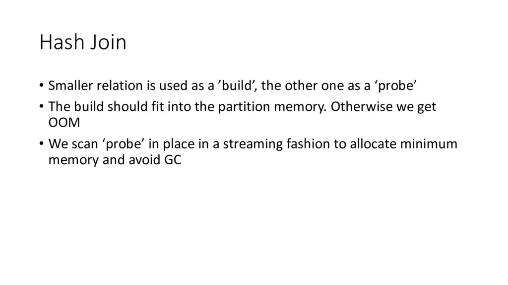
the other one as a ‘probe’ • The build should fit into the partition memory. Otherwise we get OOM • We scan ‘probe’ in place in a streaming fashion to allocate minimum memory and avoid GC
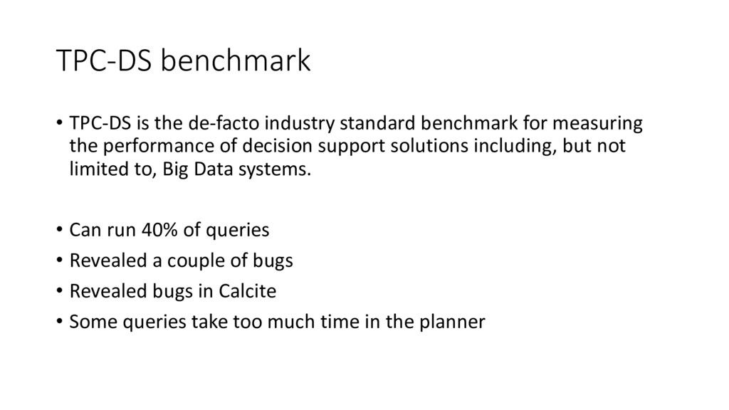
for measuring the performance of decision support solutions including, but not limited to, Big Data systems. • Can run 40% of queries • Revealed a couple of bugs • Revealed bugs in Calcite • Some queries take too much time in the planner
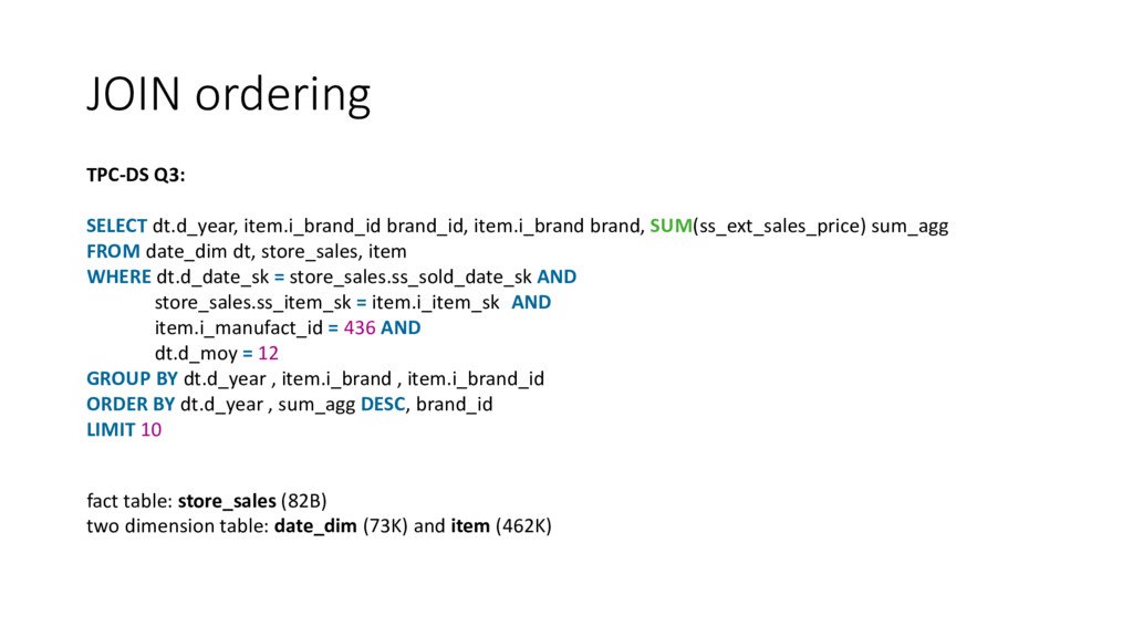
SUM(ss_ext_sales_price) sum_agg FROM date_dim dt, store_sales, item WHERE dt.d_date_sk = store_sales.ss_sold_date_sk AND store_sales.ss_item_sk = item.i_item_sk AND item.i_manufact_id = 436 AND dt.d_moy = 12 GROUP BY dt.d_year , item.i_brand , item.i_brand_id ORDER BY dt.d_year , sum_agg DESC, brand_id LIMIT 10 fact table: store_sales (82B) two dimension table: date_dim (73K) and item (462K)
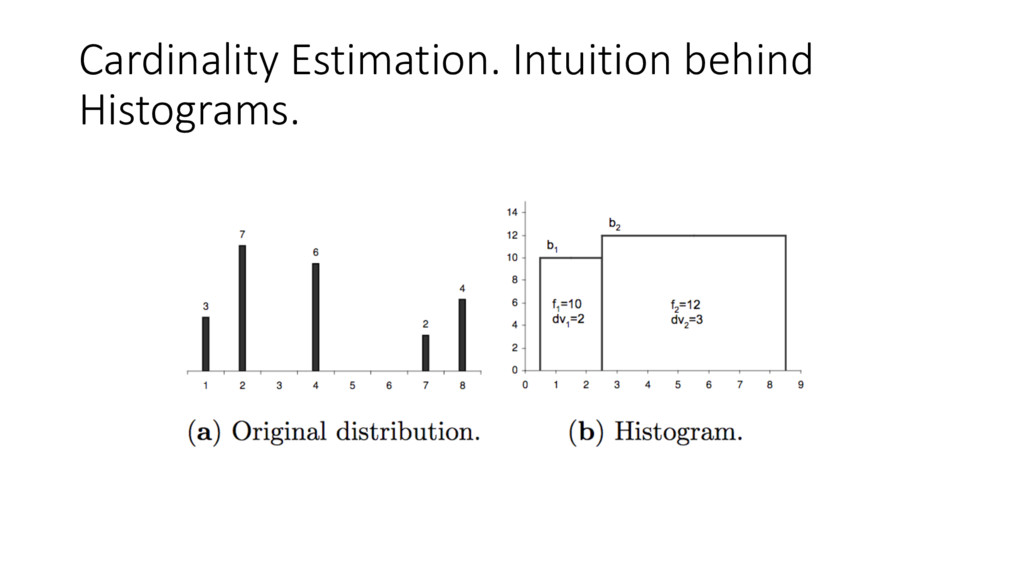
fs(a AND b) = fs(a) * fs (b) For logical-OR expression, its filter selectivity fs (a OR b) = fs (a) + fs (b) - fs (a AND b) = fs (a) + fs (b) – (fs (a) * fs (b)) For logical-NOT expression, its filter selectivity is fs (NOT a) = 1.0 - fs (a) f – number of tuples in the bucket dv – number of distinct values in the bucket