Explorando dados com Pandas

Python Day Natal 2017

Transcript

1. Explorando dados com Pandas Felipe Pontes
2. Agenda O que é pandas? Estruturas de dados Funcionalidades Integrações
3. github.com/felipemfp/python-day-natal-2017 (https:/ /github.com/felipemfp/python-day-natal- 2017)
4. O que é pandas?
5. pandas is an open source, BSD-licensed library providing high- performance, easy-to-use data structures and data analysis tools for the Python programming language
6. O que é pandas? Biblioteca open-source PANel Data System +11k no GitHub
7. numpy ndarray e matriz Acesso por índice Tipo único de dados In [117]: índice 0 1 2 3 elemento 1 3 5 7 import numpy as np arr = np.array([1, 3, 5, 7], dtype=np.int64) arr Out[117]: array([1, 3, 5, 7])
8. pandas Construído em cima do numpy Acesso por rótulo (índice ou coluna) Tipos varíados de dados
9. Por quê? Aplicável para o mundo real Estruturas de dados intuitivas Baterias inclusas para preparação, análise e exploração de dados
10. pandas no ecossistema
11. pandas no ecossistema
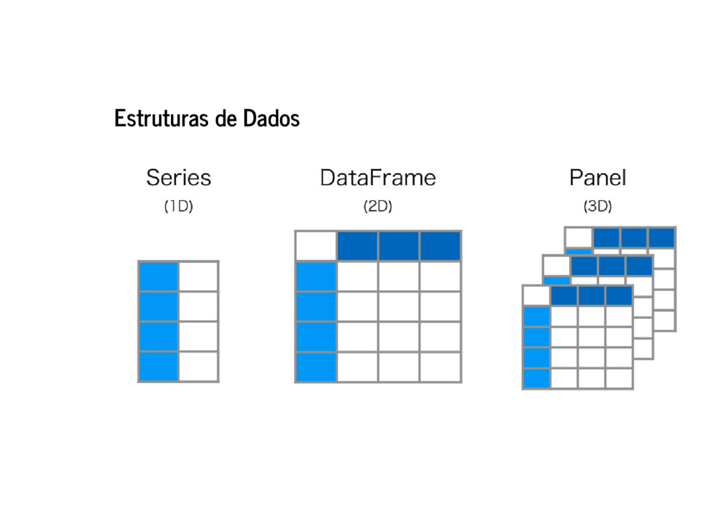
12. Estruturas de Dados In [118]: import pandas as pd
13. Estruturas de Dados
14. Series Lista rotulada de 1 dimensão Qualquer tipo de dado inteiros strings decimais objetos s = pd.Series(data, index=index)
15. Criando Series A partir de um np.ndarray In [119]: In [120]: In [121]: s = pd.Series(np.random.randn(5), index=['a', 'b', 'c', 'd', 'e']) s s.index pd.Series(np.random.randn(5)) Out[119]: a -0.363051 b 0.657138 c -1.482879 d 0.019643 e -0.009886 dtype: float64 Out[120]: Index(['a', 'b', 'c', 'd', 'e'], dtype='object') Out[121]: 0 0.158455 1 0.758866 2 -0.933195 3 0.785129 4 0.420429 dtype: float64
16. Criando Series A partir de um dict In [122]: In [123]: d = {'a' : 0., 'b' : 1., 'c' : 2.} pd.Series(d) pd.Series(d, index=['b', 'c', 'd', 'a']) NaN signi ca "Not a Number" e é um marcador padrão para valores que estão faltando. Out[122]: a 0.0 b 1.0 c 2.0 dtype: float64 Out[123]: b 1.0 c 2.0 d NaN a 0.0 dtype: float64
17. Criando Series A partir de um valor In [124]: pd.Series(5., index=['a', 'b', 'c', 'd', 'e']) Out[124]: a 5.0 b 5.0 c 5.0 d 5.0 e 5.0 dtype: float64
18. Series são como np.ndarray In [125]: In [126]: In [127]: s[0] s[:3] s[[4, 3, 1]] Out[125]: -0.3630508545612619 Out[126]: a -0.363051 b 0.657138 c -1.482879 dtype: float64 Out[127]: e -0.009886 d 0.019643 b 0.657138 dtype: float64
19. Series são como dict In [128]: In [129]: In [130]: In [131]: In [132]: s['a'] s['e'] = 12. s 'e' in s 'f' in s Out[128]: -0.3630508545612619 Out[130]: a -0.363051 b 0.657138 c -1.482879 d 0.019643 e 12.000000 dtype: float64 Out[131]: True Out[132]: False
20. Operações com Series In [133]: In [134]: In [135]: s + s s * 3 s[1:] + s[:-1] Out[133]: a -0.726102 b 1.314275 c -2.965758 d 0.039287 e 24.000000 dtype: float64 Out[134]: a -1.089153 b 1.971413 c -4.448637 d 0.058930 e 36.000000 dtype: float64 Out[135]: a NaN b 1.314275 c -2.965758 d 0.039287 e NaN dtype: float64
21. DataFrame Composição de Series Colunas com diferentes tipos df = pd.DataFrame(data, index=index)
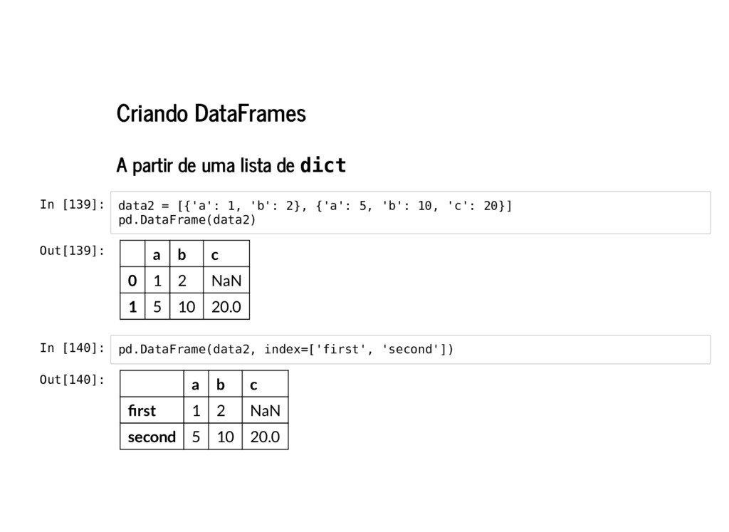
22. Criando DataFrames A partir de um dict In [136]: d = {'one' : pd.Series([1., 2., 3.], index=['a', 'b', 'c']), 'two' : pd.Series([1., 2., 3., 4.], index=['a', 'b', 'c', 'd'])} df = pd.DataFrame(d) df Out[136]: one two a 1.0 1.0 b 2.0 2.0 c 3.0 3.0 d NaN 4.0
23. Criando DataFrames A partir de um dict In [137]: In [138]: pd.DataFrame(d, index=['d', 'b', 'a']) pd.DataFrame(d, index=['d', 'b', 'a'], columns=['two', 'three']) Out[137]: one two d NaN 4.0 b 2.0 2.0 a 1.0 1.0 Out[138]: two three d 4.0 NaN b 2.0 NaN a 1.0 NaN
24. Criando DataFrames A partir de uma lista de dict In [139]: In [140]: data2 = [{'a': 1, 'b': 2}, {'a': 5, 'b': 10, 'c': 20}] pd.DataFrame(data2) pd.DataFrame(data2, index=['first', 'second']) Out[139]: a b c 0 1 2 NaN 1 5 10 20.0 Out[140]: a b c rst 1 2 NaN second 5 10 20.0
25. Criando DataFrames A partir de uma Series Mantém os índices Uma coluna com nome da Series ou argumento passado
26. Operações com DataFrame Projeção In [141]: Adição In [142]: df['one'] df['three'] = df['one'] * df['two'] df['flag'] = df['one'] > 2 df Out[141]: a 1.0 b 2.0 c 3.0 d NaN Name: one, dtype: float64 Out[142]: one two three ag a 1.0 1.0 1.0 False b 2.0 2.0 4.0 False c 3.0 3.0 9.0 True d NaN 4.0 NaN False
27. In [143]: df['foo'] = 'bar' df Out[143]: one two three ag foo a 1.0 1.0 1.0 False bar b 2.0 2.0 4.0 False bar c 3.0 3.0 9.0 True bar d NaN 4.0 NaN False bar
28. Operações com DataFrame Exclusão In [144]: In [145]: del df['two'] three = df.pop('three') df Out[145]: one ag foo a 1.0 False bar b 2.0 False bar c 3.0 True bar d NaN False bar
29. Panel Composição de DataFrames Descontinuado
30. Funcionalidades
31. Criando objetos In [146]: s = pd.Series([1,3,5,np.nan,6,8]) s Out[146]: 0 1.0 1 3.0 2 5.0 3 NaN 4 6.0 5 8.0 dtype: float64
32. Criando objetos In [147]: In [148]: dates = pd.date_range('20130101', periods=6) dates df = pd.DataFrame(np.random.randn(6,4), index=dates, columns=list('ABCD')) df Out[147]: DatetimeIndex(['2013-01-01', '2013-01-02', '2013-01-03', '2013-01-04', '2013-01-05', '2013-01-06'], dtype='datetime64[ns]', freq='D') Out[148]: A B C D 2013-01-01 0.942514 0.457859 1.796804 -0.167335 2013-01-02 1.350054 0.372804 1.179525 -1.497362 2013-01-03 1.396315 1.669783 0.014493 0.069263 2013-01-04 -1.512057 -0.942973 -0.142368 -0.042194 2013-01-05 -0.302740 -1.613105 2.650310 1.237520 2013-01-06 1.338176 -0.302371 0.908058 2.669694
33. Criando objetos In [149]: df2 = pd.DataFrame({ 'A' : 1., 'B' : pd.Timestamp('20130102'), 'C' : pd.Series(1,index=list(range(4)),dtype='float32'), 'D' : np.array([3] * 4,dtype='int32'), 'E' : pd.Categorical(["test","train","test","train"]), 'F' : 'foo' }) df2 Out[149]: A B C D E F 0 1.0 2013-01-02 1.0 3 test foo 1 1.0 2013-01-02 1.0 3 train foo 2 1.0 2013-01-02 1.0 3 test foo 3 1.0 2013-01-02 1.0 3 train foo
34. Entendendo os dados In [150]: In [151]: df.head() df.tail(3) Out[150]: A B C D 2013-01-01 0.942514 0.457859 1.796804 -0.167335 2013-01-02 1.350054 0.372804 1.179525 -1.497362 2013-01-03 1.396315 1.669783 0.014493 0.069263 2013-01-04 -1.512057 -0.942973 -0.142368 -0.042194 2013-01-05 -0.302740 -1.613105 2.650310 1.237520 Out[151]: A B C D 2013-01-04 -1.512057 -0.942973 -0.142368 -0.042194 2013-01-05 -0.302740 -1.613105 2.650310 1.237520 2013-01-06 1.338176 -0.302371 0.908058 2.669694
35. Entendendo os dados In [152]: In [153]: In [154]: df.index df.columns df.values Out[152]: DatetimeIndex(['2013-01-01', '2013-01-02', '2013-01-03', '2013-01-04', '2013-01-05', '2013-01-06'], dtype='datetime64[ns]', freq='D') Out[153]: Index(['A', 'B', 'C', 'D'], dtype='object') Out[154]: array([[ 0.94251405, 0.45785949, 1.79680407, -0.1673346 ], [ 1.350054 , 0.37280432, 1.17952484, -1.49736159], [ 1.39631522, 1.66978288, 0.01449329, 0.0692628 ], [-1.51205691, -0.94297288, -0.14236803, -0.0421941 ], [-0.30273957, -1.61310536, 2.65031003, 1.2375204 ], [ 1.33817644, -0.3023708 , 0.90805789, 2.66969448]])
36. Entendendo os dados In [155]: df.describe() Out[155]: A B C D count 6.000000 6.000000 6.000000 6.000000 mean 0.535377 -0.059667 1.067804 0.378265 std 1.192442 1.157425 1.062803 1.419640 min -1.512057 -1.613105 -0.142368 -1.497362 25% 0.008574 -0.782822 0.237884 -0.136049 50% 1.140345 0.035217 1.043791 0.013534 75% 1.347085 0.436596 1.642484 0.945456 max 1.396315 1.669783 2.650310 2.669694
37. Entendendo os dados In [156]: df.info() <class 'pandas.core.frame.DataFrame'> DatetimeIndex: 6 entries, 2013-01-01 to 2013-01-06 Freq: D Data columns (total 4 columns): A 6 non-null float64 B 6 non-null float64 C 6 non-null float64 D 6 non-null float64 dtypes: float64(4) memory usage: 240.0 bytes
38. Manipulando os dados Obtendo a transposta In [157]: df.T Out[157]: 2013-01- 01 00:00:00 2013-01- 02 00:00:00 2013-01- 03 00:00:00 2013-01- 04 00:00:00 2013-01- 05 00:00:00 2013-01- 06 00:00:00 A 0.942514 1.350054 1.396315 -1.512057 -0.302740 1.338176 B 0.457859 0.372804 1.669783 -0.942973 -1.613105 -0.302371 C 1.796804 1.179525 0.014493 -0.142368 2.650310 0.908058 D -0.167335 -1.497362 0.069263 -0.042194 1.237520 2.669694
39. Manipulando os dados Ordenando índices In [158]: df.sort_index(axis=1, ascending=False) Out[158]: D C B A 2013-01-01 -0.167335 1.796804 0.457859 0.942514 2013-01-02 -1.497362 1.179525 0.372804 1.350054 2013-01-03 0.069263 0.014493 1.669783 1.396315 2013-01-04 -0.042194 -0.142368 -0.942973 -1.512057 2013-01-05 1.237520 2.650310 -1.613105 -0.302740 2013-01-06 2.669694 0.908058 -0.302371 1.338176
40. Manipulando os dados Ordenando valores In [159]: df.sort_values(by='B') Out[159]: A B C D 2013-01-05 -0.302740 -1.613105 2.650310 1.237520 2013-01-04 -1.512057 -0.942973 -0.142368 -0.042194 2013-01-06 1.338176 -0.302371 0.908058 2.669694 2013-01-02 1.350054 0.372804 1.179525 -1.497362 2013-01-01 0.942514 0.457859 1.796804 -0.167335 2013-01-03 1.396315 1.669783 0.014493 0.069263
41. Projetando os dados In [160]: df['A'] Out[160]: 2013-01-01 0.942514 2013-01-02 1.350054 2013-01-03 1.396315 2013-01-04 -1.512057 2013-01-05 -0.302740 2013-01-06 1.338176 Freq: D, Name: A, dtype: float64
42. Projetando os dados In [161]: In [162]: df[0:3] df['20130102':'20130104'] Out[161]: A B C D 2013-01-01 0.942514 0.457859 1.796804 -0.167335 2013-01-02 1.350054 0.372804 1.179525 -1.497362 2013-01-03 1.396315 1.669783 0.014493 0.069263 Out[162]: A B C D 2013-01-02 1.350054 0.372804 1.179525 -1.497362 2013-01-03 1.396315 1.669783 0.014493 0.069263 2013-01-04 -1.512057 -0.942973 -0.142368 -0.042194
43. Projetando os dados Por rótulo In [163]: df.loc[dates[0]] Out[163]: A 0.942514 B 0.457859 C 1.796804 D -0.167335 Name: 2013-01-01 00:00:00, dtype: float64
44. Projetando os dados Por rótulo In [164]: df.loc[:,['A','B']] Out[164]: A B 2013-01-01 0.942514 0.457859 2013-01-02 1.350054 0.372804 2013-01-03 1.396315 1.669783 2013-01-04 -1.512057 -0.942973 2013-01-05 -0.302740 -1.613105 2013-01-06 1.338176 -0.302371
45. Projetando os dados Por rótulo In [165]: df.loc['20130102':'20130104',['A','B']] Out[165]: A B 2013-01-02 1.350054 0.372804 2013-01-03 1.396315 1.669783 2013-01-04 -1.512057 -0.942973
46. Projetando os dados Por rótulo In [166]: In [167]: df.loc['20130102',['A','B']] df.loc[dates[0],'A'] Out[166]: A 1.350054 B 0.372804 Name: 2013-01-02 00:00:00, dtype: float64 Out[167]: 0.94251404675651695
47. Projetando os dados Por posição In [168]: In [169]: df.iloc[3] df.iloc[3:5,0:2] Out[168]: A -1.512057 B -0.942973 C -0.142368 D -0.042194 Name: 2013-01-04 00:00:00, dtype: float64 Out[169]: A B 2013-01-04 -1.512057 -0.942973 2013-01-05 -0.302740 -1.613105
48. Projetando os dados Por posição In [170]: In [171]: df.iloc[[1,2,4],[0,2]] df.iloc[1:3,:] Out[170]: A C 2013-01-02 1.350054 1.179525 2013-01-03 1.396315 0.014493 2013-01-05 -0.302740 2.650310 Out[171]: A B C D 2013-01-02 1.350054 0.372804 1.179525 -1.497362 2013-01-03 1.396315 1.669783 0.014493 0.069263
49. Projetando os dados Por posição In [172]: In [173]: df.iloc[:,1:3] df.iloc[1,1] Out[172]: B C 2013-01-01 0.457859 1.796804 2013-01-02 0.372804 1.179525 2013-01-03 1.669783 0.014493 2013-01-04 -0.942973 -0.142368 2013-01-05 -1.613105 2.650310 2013-01-06 -0.302371 0.908058 Out[173]: 0.37280432445655604
50. Projetando os dados Por condição In [174]: In [175]: df[df.A > 0] df[df > 0] Out[174]: A B C D 2013-01-01 0.942514 0.457859 1.796804 -0.167335 2013-01-02 1.350054 0.372804 1.179525 -1.497362 2013-01-03 1.396315 1.669783 0.014493 0.069263 2013-01-06 1.338176 -0.302371 0.908058 2.669694 Out[175]: A B C D 2013-01-01 0.942514 0.457859 1.796804 NaN 2013-01-02 1.350054 0.372804 1.179525 NaN 2013-01-03 1.396315 1.669783 0.014493 0.069263 2013-01-04 NaN NaN NaN NaN 2013-01-05 NaN NaN 2.650310 1.237520 2013-01-06 1.338176 NaN 0.908058 2.669694
51. Projetando os dados isin() In [176]: In [177]: df2 = df.copy() df2['E'] = ['one', 'one','two','three','four','three'] df2 df2[df2['E'].isin(['two','four'])] Out[176]: A B C D E 2013-01-01 0.942514 0.457859 1.796804 -0.167335 one 2013-01-02 1.350054 0.372804 1.179525 -1.497362 one 2013-01-03 1.396315 1.669783 0.014493 0.069263 two 2013-01-04 -1.512057 -0.942973 -0.142368 -0.042194 three 2013-01-05 -0.302740 -1.613105 2.650310 1.237520 four 2013-01-06 1.338176 -0.302371 0.908058 2.669694 three Out[177]: A B C D E 2013-01-03 1.396315 1.669783 0.014493 0.069263 two 2013-01-05 -0.302740 -1.613105 2.650310 1.237520 four
52. Modi cando os dados Adicionando colunas In [178]: In [179]: s1 = pd.Series([1,2,3,4,5,6], index=pd.date_range('20130102', periods=6)) s1 df['F'] = s1 Out[178]: 2013-01-02 1 2013-01-03 2 2013-01-04 3 2013-01-05 4 2013-01-06 5 2013-01-07 6 Freq: D, dtype: int64
53. Modi cando os dados Alterando valores In [180]: df Out[180]: A B C D F 2013-01-01 0.942514 0.457859 1.796804 -0.167335 NaN 2013-01-02 1.350054 0.372804 1.179525 -1.497362 1.0 2013-01-03 1.396315 1.669783 0.014493 0.069263 2.0 2013-01-04 -1.512057 -0.942973 -0.142368 -0.042194 3.0 2013-01-05 -0.302740 -1.613105 2.650310 1.237520 4.0 2013-01-06 1.338176 -0.302371 0.908058 2.669694 5.0
54. Modi cando os dados Alterando valores In [181]: df.at[dates[0],'A'] = 0 df.iat[0,1] = 0 df.loc[:,'D'] = np.array([5] * len(df)) df Out[181]: A B C D F 2013-01-01 0.000000 0.000000 1.796804 5 NaN 2013-01-02 1.350054 0.372804 1.179525 5 1.0 2013-01-03 1.396315 1.669783 0.014493 5 2.0 2013-01-04 -1.512057 -0.942973 -0.142368 5 3.0 2013-01-05 -0.302740 -1.613105 2.650310 5 4.0 2013-01-06 1.338176 -0.302371 0.908058 5 5.0
55. Modi cando os dados Alterando valores com condições In [182]: df2 = df.copy() df2 Out[182]: A B C D F 2013-01-01 0.000000 0.000000 1.796804 5 NaN 2013-01-02 1.350054 0.372804 1.179525 5 1.0 2013-01-03 1.396315 1.669783 0.014493 5 2.0 2013-01-04 -1.512057 -0.942973 -0.142368 5 3.0 2013-01-05 -0.302740 -1.613105 2.650310 5 4.0 2013-01-06 1.338176 -0.302371 0.908058 5 5.0
56. Modi cando os dados Alterando valores com condições In [183]: df2[df2 > 0] = -df2 df2 Out[183]: A B C D F 2013-01-01 0.000000 0.000000 -1.796804 -5 NaN 2013-01-02 -1.350054 -0.372804 -1.179525 -5 -1.0 2013-01-03 -1.396315 -1.669783 -0.014493 -5 -2.0 2013-01-04 -1.512057 -0.942973 -0.142368 -5 -3.0 2013-01-05 -0.302740 -1.613105 -2.650310 -5 -4.0 2013-01-06 -1.338176 -0.302371 -0.908058 -5 -5.0
57. Tratando os dados In [184]: df1 = df.reindex(index=dates[0:4], columns=list(df.columns) + ['E']) df1.loc[dates[0]:dates[1],'E'] = 1 df1 Out[184]: A B C D F E 2013-01-01 0.000000 0.000000 1.796804 5 NaN 1.0 2013-01-02 1.350054 0.372804 1.179525 5 1.0 1.0 2013-01-03 1.396315 1.669783 0.014493 5 2.0 NaN 2013-01-04 -1.512057 -0.942973 -0.142368 5 3.0 NaN
58. Tratando os dados In [185]: In [186]: df1 pd.isnull(df1) Out[185]: A B C D F E 2013-01-01 0.000000 0.000000 1.796804 5 NaN 1.0 2013-01-02 1.350054 0.372804 1.179525 5 1.0 1.0 2013-01-03 1.396315 1.669783 0.014493 5 2.0 NaN 2013-01-04 -1.512057 -0.942973 -0.142368 5 3.0 NaN Out[186]: A B C D F E 2013-01-01 False False False False True False 2013-01-02 False False False False False False 2013-01-03 False False False False False True 2013-01-04 False False False False False True
59. Tratando os dados In [187]: In [188]: df1.dropna(how='any') df1.fillna(value=5) Out[187]: A B C D F E 2013-01-02 1.350054 0.372804 1.179525 5 1.0 1.0 Out[188]: A B C D F E 2013-01-01 0.000000 0.000000 1.796804 5 5.0 1.0 2013-01-02 1.350054 0.372804 1.179525 5 1.0 1.0 2013-01-03 1.396315 1.669783 0.014493 5 2.0 5.0 2013-01-04 -1.512057 -0.942973 -0.142368 5 3.0 5.0
60. Tratando os dados apply() In [189]: In [190]: df.apply(np.cumsum) df.apply(lambda x: x.max() - x.min()) Out[189]: A B C D F 2013-01-01 0.000000 0.000000 1.796804 5 NaN 2013-01-02 1.350054 0.372804 2.976329 10 1.0 2013-01-03 2.746369 2.042587 2.990822 15 3.0 2013-01-04 1.234312 1.099614 2.848454 20 6.0 2013-01-05 0.931573 -0.513491 5.498764 25 10.0 2013-01-06 2.269749 -0.815862 6.406822 30 15.0 Out[190]: A 2.908372 B 3.282888 C 2.792678 D 0.000000 F 4.000000 dtype: float64
61. Tratando os dados apply() In [191]: df.apply(lambda x: [max(1, y) for y in x]) Out[191]: A B C D F 2013-01-01 1.000000 1.000000 1.796804 5 1.0 2013-01-02 1.350054 1.000000 1.179525 5 1.0 2013-01-03 1.396315 1.669783 1.000000 5 2.0 2013-01-04 1.000000 1.000000 1.000000 5 3.0 2013-01-05 1.000000 1.000000 2.650310 5 4.0 2013-01-06 1.338176 1.000000 1.000000 5 5.0
62. Operando com os dados Estatísticas In [192]: df.mean() Out[192]: A 0.378292 B -0.135977 C 1.067804 D 5.000000 F 3.000000 dtype: float64
63. Operando com os dados Estatísticas In [193]: df.mean(1) Out[193]: 2013-01-01 1.699201 2013-01-02 1.780477 2013-01-03 2.016118 2013-01-04 1.080520 2013-01-05 1.946893 2013-01-06 2.388773 Freq: D, dtype: float64
64. Operando com os dados Estatísticas In [194]: In [195]: s = pd.Series(np.random.randint(0, 7, size=10)) s s.value_counts() Out[194]: 0 4 1 4 2 5 3 5 4 4 5 1 6 1 7 5 8 5 9 5 dtype: int64 Out[195]: 5 5 4 3 1 2 dtype: int64
65. Operando com os dados Strings In [196]: In [197]: s = pd.Series(['A', 'B', 'C', 'Aaba', 'Baca', np.nan, 'CABA', 'dog', 'cat']) s s.str.lower() Out[196]: 0 A 1 B 2 C 3 Aaba 4 Baca 5 NaN 6 CABA 7 dog 8 cat dtype: object Out[197]: 0 a 1 b 2 c 3 aaba 4 baca 5 NaN 6 caba 7 dog 8 cat dtype: object
66. Mesclando dados Merge In [198]: df = pd.DataFrame(np.random.randn(10, 4)) df Out[198]: 0 1 2 3 0 -0.616159 0.441333 0.644670 2.336805 1 -0.474553 -0.398493 1.424062 -0.877346 2 -0.253474 0.265718 -2.457648 -0.231814 3 0.079574 1.797657 -0.527753 1.333898 4 -0.098189 1.196968 0.249564 -1.927953 5 -1.621114 0.080282 -0.089616 2.160123 6 0.181398 0.837641 -0.553422 -0.998054 7 0.527065 0.750490 0.248069 -0.480715 8 1.673566 0.408616 -0.297147 0.400781 9 0.711653 1.887566 -0.340432 0.284253
67. Mesclando dados Merge In [199]: pieces = [df[:3], df[3:7], df[7:]] pd.concat(pieces) Out[199]: 0 1 2 3 0 -0.616159 0.441333 0.644670 2.336805 1 -0.474553 -0.398493 1.424062 -0.877346 2 -0.253474 0.265718 -2.457648 -0.231814 3 0.079574 1.797657 -0.527753 1.333898 4 -0.098189 1.196968 0.249564 -1.927953 5 -1.621114 0.080282 -0.089616 2.160123 6 0.181398 0.837641 -0.553422 -0.998054 7 0.527065 0.750490 0.248069 -0.480715 8 1.673566 0.408616 -0.297147 0.400781 9 0.711653 1.887566 -0.340432 0.284253
68. Mesclando dados Join In [200]: In [201]: In [202]: left = pd.DataFrame({'key': ['foo', 'foo'], 'lval': [1, 2]}) right = pd.DataFrame({'key': ['foo', 'foo'], 'rval': [4, 5]}) left right Out[201]: key lval 0 foo 1 1 foo 2 Out[202]: key rval 0 foo 4 1 foo 5
69. Mesclando dados Join In [203]: pd.merge(left, right, on='key') Out[203]: key lval rval 0 foo 1 4 1 foo 1 5 2 foo 2 4 3 foo 2 5
70. Mesclando dados Append In [204]: df = pd.DataFrame(np.random.randn(8, 4), columns=['A','B','C','D']) df Out[204]: A B C D 0 -0.309317 0.244977 0.881038 0.138781 1 -1.930083 -0.680669 -1.452549 -0.150607 2 2.116961 -0.544347 -0.604566 -0.793241 3 -0.740517 0.088858 -0.119330 0.475188 4 1.724797 0.682759 0.165117 0.298184 5 0.505510 -1.446364 -1.630013 0.015845 6 0.416764 0.448405 0.746967 -0.059918 7 0.950208 -0.010430 0.167761 -0.325940
71. Mesclando dados Append In [205]: s = df.iloc[3] s Out[205]: A -0.740517 B 0.088858 C -0.119330 D 0.475188 Name: 3, dtype: float64
72. Mesclando dados Append In [206]: df.append(s, ignore_index=True) Out[206]: A B C D 0 -0.309317 0.244977 0.881038 0.138781 1 -1.930083 -0.680669 -1.452549 -0.150607 2 2.116961 -0.544347 -0.604566 -0.793241 3 -0.740517 0.088858 -0.119330 0.475188 4 1.724797 0.682759 0.165117 0.298184 5 0.505510 -1.446364 -1.630013 0.015845 6 0.416764 0.448405 0.746967 -0.059918 7 0.950208 -0.010430 0.167761 -0.325940 8 -0.740517 0.088858 -0.119330 0.475188
73. Agrupando dados In [207]: df = pd.DataFrame({'A' : ['foo', 'bar', 'foo', 'bar', 'foo', 'bar', 'foo', 'foo'], 'B' : ['one', 'one', 'two', 'three', 'two', 'two', 'one', 'three'], 'C' : np.random.randn(8), 'D' : np.random.randn(8)}) df Out[207]: A B C D 0 foo one 0.329304 -1.481057 1 bar one 1.123981 -1.507624 2 foo two -0.277149 -0.110525 3 bar three 1.013107 1.072455 4 foo two -0.263508 0.635959 5 bar two -0.210274 -0.015596 6 foo one -1.456826 1.875040 7 foo three -1.748910 -0.674866
74. Agrupando dados In [208]: df.groupby('A').sum() Out[208]: C D A bar 1.926814 -0.450765 foo -3.417090 0.244550
75. Agrupando dados In [209]: df.groupby(['A','B']).sum() Out[209]: C D A B bar one 1.123981 -1.507624 three 1.013107 1.072455 two -0.210274 -0.015596 foo one -1.127522 0.393983 three -1.748910 -0.674866 two -0.540658 0.525433
76. Integrações In [211]: import matplotlib.pyplot as plt
77. Matplotlib In [212]: ts = pd.Series(np.random.randn(1000), index=pd.date_range('1/1/2000', periods=1 000)) ts = ts.cumsum() ts.plot() Out[212]: <matplotlib.axes._subplots.AxesSubplot at 0x7f184c87aa58>
78. Matplotlib In [213]: df = pd.DataFrame(np.random.randn(1000, 4), index=ts.index, columns=['A', 'B', 'C', 'D']) df = df.cumsum() plt.figure(); df.plot(); plt.legend(loc='best') Out[213]: <matplotlib.legend.Legend at 0x7f184c71e898> <matplotlib.figure.Figure at 0x7f184f51fa58>
79. CSV In [214]: In [215]: df.to_csv('data/foo.csv', index_label='date') df = pd.read_csv('data/foo.csv', index_col='date') df.head() Out[215]: A B C D date 2000-01-01 -0.184042 0.174102 0.940474 -0.233452 2000-01-02 -0.126755 -0.524672 1.917568 0.571711 2000-01-03 -1.624824 -1.536377 2.817070 0.980146 2000-01-04 -1.535097 -1.367084 2.275337 0.119631 2000-01-05 -0.450131 -1.138307 2.793651 1.284019
80. HDF5 In [216]: In [217]: df.to_hdf('data/foo.h5','df') df = pd.read_hdf('data/foo.h5','df') df.head() Out[217]: A B C D date 2000-01-01 -0.184042 0.174102 0.940474 -0.233452 2000-01-02 -0.126755 -0.524672 1.917568 0.571711 2000-01-03 -1.624824 -1.536377 2.817070 0.980146 2000-01-04 -1.535097 -1.367084 2.275337 0.119631 2000-01-05 -0.450131 -1.138307 2.793651 1.284019
81. Excel In [218]: In [219]: df.to_excel('data/foo.xlsx', index_label='date', sheet_name='Sheet1') df = pd.read_excel('data/foo.xlsx', 'Sheet1', index_col='date', na_values=['NA' ]) df.head() Out[219]: A B C D date 2000-01-01 -0.184042 0.174102 0.940474 -0.233452 2000-01-02 -0.126755 -0.524672 1.917568 0.571711 2000-01-03 -1.624824 -1.536377 2.817070 0.980146 2000-01-04 -1.535097 -1.367084 2.275337 0.119631 2000-01-05 -0.450131 -1.138307 2.793651 1.284019
82. Obrigado! Dúvidas? Felipe Pontes @felipemfp felipemfpontes@gmail.com
83. Links Intro to Data Structures (http://pandas.pydata.org/pandas- docs/stable/dsintro.html) 10 Minutes to pandas (http://pandas.pydata.org/pandas- docs/stable/10min.html) PyConJP 2015: pandas internals by Sinhrks (https://speakerdeck.com/sinhrks/pyconjp-2015-pandas-internals) Pandas for Data Analysis by phanhoang17 (https://speakerdeck.com/huyhoang17/pandas-for-data-analysis)