MCQMC 2018 July 4 Rennes

Minisymposium talk on when to stop a simulation, comparing Bayesian and deterministic perspectives and illustrating how to use fast transforms with low discrepancy designs

Transcript

1. Fast Adaptive Bayesian Cubature Using Low Discrepancy Sampling: A Cross-Cultural Talk Fred J. Hickernell and R. Jagadeeswaran Department of Applied Mathematics Center for Interdisciplinary Scientific Computation Illinois Institute of Technology hickernell@iit.edu mypages.iit.edu/~hickernell Thanks to the GAIL team, NSF-DMS-1522687 and NSF-DMS-1638521 (SAMSI) Monte Carlo and Quasi-Monte Carlo Methods, July 4, 2018
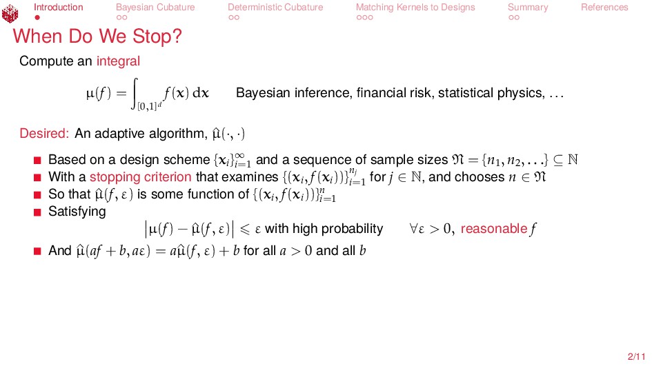
2. Introduction Bayesian Cubature Deterministic Cubature Matching Kernels to Designs Summary References When Do We Stop? Compute an integral µ(f) = [0,1]d f(x) dx Bayesian inference, financial risk, statistical physics, ... Desired: An adaptive algorithm, ^ µ(·, ·) Based on a design scheme {xi }∞ i=1 and a sequence of sample sizes N = {n1 , n2 , . . .} ⊆ N With a stopping criterion that examines {(xi , f(xi ))}nj i=1 for j ∈ N, and chooses n ∈ N So that ^ µ(f, ε) is some function of {(xi , f(xi ))}n i=1 Satisfying µ(f) − ^ µ(f, ε) ε with high probability ∀ε > 0, reasonable f And ^ µ(af + b, aε) = a^ µ(f, ε) + b for all a > 0 and all b 2/11
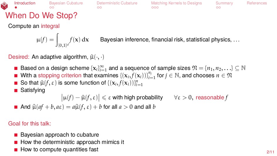
3. Introduction Bayesian Cubature Deterministic Cubature Matching Kernels to Designs Summary References When Do We Stop? Compute an integral µ(f) = [0,1]d f(x) dx Bayesian inference, financial risk, statistical physics, ... Desired: An adaptive algorithm, ^ µ(·, ·) Based on a design scheme {xi }∞ i=1 and a sequence of sample sizes N = {n1 , n2 , . . .} ⊆ N With a stopping criterion that examines {(xi , f(xi ))}nj i=1 for j ∈ N, and chooses n ∈ N So that ^ µ(f, ε) is some function of {(xi , f(xi ))}n i=1 Satisfying µ(f) − ^ µ(f, ε) ε with high probability ∀ε > 0, reasonable f And ^ µ(af + b, aε) = a^ µ(f, ε) + b for all a > 0 and all b Goal for this talk: Bayesian approach to cubature How the deterministic approach mimics it How to compute quantities fast 2/11
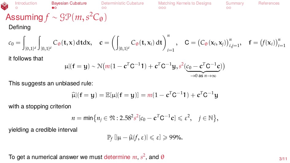
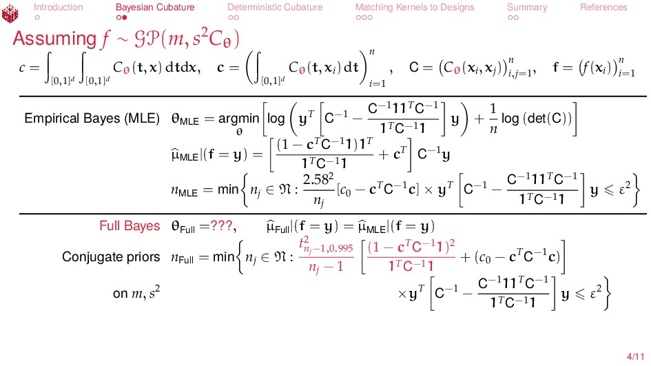
4. Introduction Bayesian Cubature Deterministic Cubature Matching Kernels to Designs Summary References Assuming f ∼ GP(m, s2Cθ ) Defining c0 = [0,1]d [0,1]d Cθ(t, x) dtdx, c = [0,1]d Cθ(t, xi ) dt n i=1 , C = Cθ(xi , xj ) n i,j=1 , f = f(xi ) n i=1 it follows that µ|(f = y) ∼ N m(1 − cTC−11) + cTC−1y, s2(c0 − cTC−1c →0 as n→∞ ) This suggests an unbiased rule: µ|(f = y) = E[µ|(f = y)] = m(1 − cTC−11) + cTC−1y with a stopping criterion n = min nj ∈ N : 2.582s2[c0 − cTC−1c] ε2, j ∈ N , yielding a credible interval Pf [|µ − ^ µ(f, ε)| ε] 99%. To get a numerical answer we must determine m, s2, and θ 3/11
5. Introduction Bayesian Cubature Deterministic Cubature Matching Kernels to Designs Summary References Assuming f ∼ GP(m, s2Cθ ) c = [0,1]d [0,1]d Cθ(t, x) dtdx, c = [0,1]d Cθ(t, xi ) dt n i=1 , C = Cθ(xi , xj ) n i,j=1 , f = f(xi ) n i=1 Empirical Bayes (MLE) θMLE = argmin θ log yT C−1 − C−111TC−1 1TC−11 y + 1 n log (det(C)) µMLE |(f = y) = (1 − cTC−11)1T 1TC−11 + cT C−1y nMLE = min nj ∈ N : 2.582 nj [c0 − cTC−1c] × yT C−1 − C−111TC−1 1TC−11 y ε2 4/11
6. Introduction Bayesian Cubature Deterministic Cubature Matching Kernels to Designs Summary References Assuming f ∼ GP(m, s2Cθ ) c = [0,1]d [0,1]d Cθ(t, x) dtdx, c = [0,1]d Cθ(t, xi ) dt n i=1 , C = Cθ(xi , xj ) n i,j=1 , f = f(xi ) n i=1 Empirical Bayes (MLE) θMLE = argmin θ log yT C−1 − C−111TC−1 1TC−11 y + 1 n log (det(C)) µMLE |(f = y) = (1 − cTC−11)1T 1TC−11 + cT C−1y nMLE = min nj ∈ N : 2.582 nj [c0 − cTC−1c] × yT C−1 − C−111TC−1 1TC−11 y ε2 Full Bayes θFull =???, µFull |(f = y) = µMLE |(f = y) Conjugate priors nFull = min nj ∈ N : t2 nj−1,0.995 nj − 1 (1 − cTC−11)2 1TC−11 + (c0 − cTC−1c) on m, s2 ×yT C−1 − C−111TC−1 1TC−11 y ε2 4/11
7. Introduction Bayesian Cubature Deterministic Cubature Matching Kernels to Designs Summary References Assuming f ∼ GP(m, s2Cθ ) Empirical Bayes (MLE) θMLE = argmin θ log yT C−1 − C−111TC−1 1TC−11 y + 1 n log (det(C)) µMLE |(f = y) = (1 − cTC−11)1T 1TC−11 + cT C−1y nMLE = min nj ∈ N : 2.582 nj [c0 − cTC−1c] × yT C−1 − C−111TC−1 1TC−11 y ε2 Full Bayes θFull =???, µFull |(f = y) = µMLE |(f = y) Conjugate priors nFull = min nj ∈ N : t2 nj−1,0.995 nj − 1 (1 − cTC−11)2 1TC−11 + (c0 − cTC−1c) on m, s2 ×yT C−1 − C−111TC−1 1TC−11 y ε2 Generalized s2 GCV =???, µGCV |(f = y) = (1 − cTC−11)1TC−1 1TC−21 + cT C−1y Cross Validation θGCV = argmin θ log yT C−2 − C−211TC−2 1TC−21 y − 2 log trace(C−1) 4/11
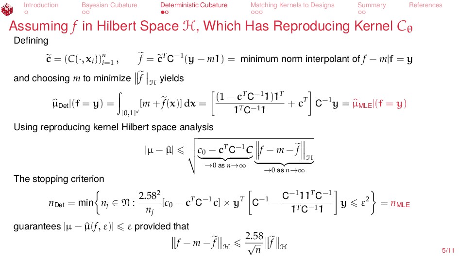
8. Introduction Bayesian Cubature Deterministic Cubature Matching Kernels to Designs Summary References Assuming f in Hilbert Space H, Which Has Reproducing Kernel Cθ Defining c = (C(·, xi ))n i=1 , f = cTC−1(y − m1) = minimum norm interpolant of f − m|f = y and choosing m to minimize f H yields µDet |(f = y) = [0,1]d [m + f(x)] dx = (1 − cTC−11)1T 1TC−11 + cT C−1y = µMLE |(f = y) Using reproducing kernel Hilbert space analysis |µ − ^ µ| c0 − cTC−1C →0 as n→∞ f − m − f H →0 as n→∞ The stopping criterion nDet = min nj ∈ N : 2.582 nj [c0 − cTC−1c] × yT C−1 − C−111TC−1 1TC−11 y ε2 = nMLE guarantees |µ − ^ µ(f, ε)| ε provided that f − m − f H 2.58 √ n f H 5/11
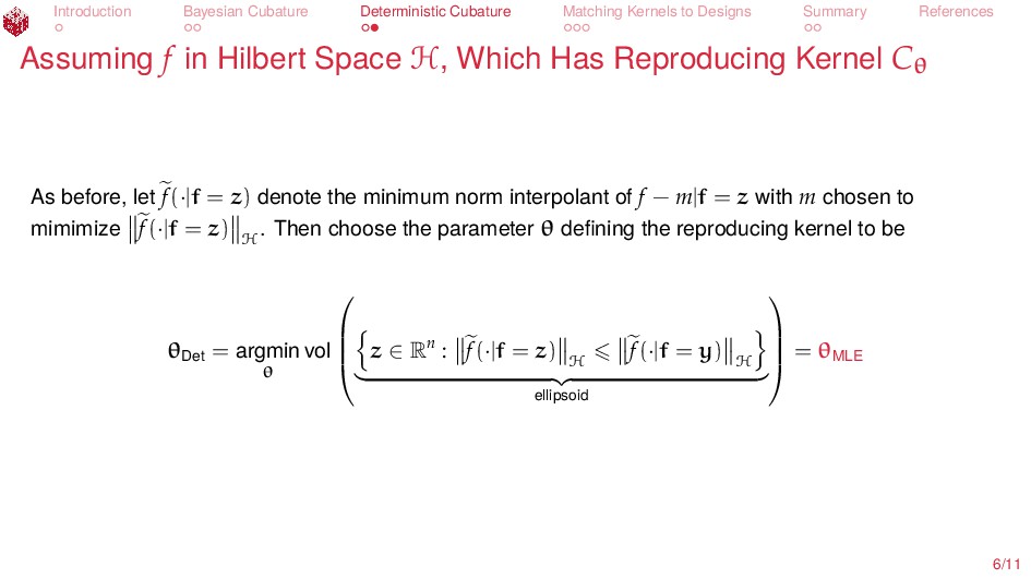
9. Introduction Bayesian Cubature Deterministic Cubature Matching Kernels to Designs Summary References Assuming f in Hilbert Space H, Which Has Reproducing Kernel Cθ As before, let f(·|f = z) denote the minimum norm interpolant of f − m|f = z with m chosen to mimimize f(·|f = z) H . Then choose the parameter θ defining the reproducing kernel to be θDet = argmin θ vol     z ∈ Rn : f(·|f = z) H f(·|f = y) H ellipsoid     = θMLE 6/11
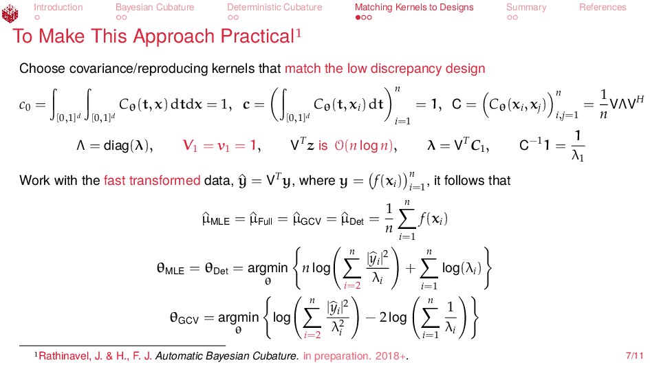
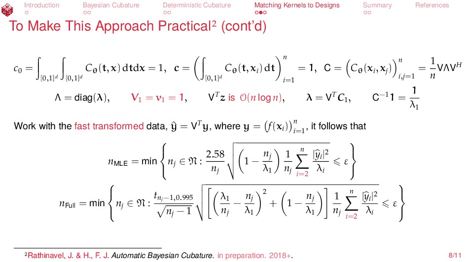
10. Introduction Bayesian Cubature Deterministic Cubature Matching Kernels to Designs Summary References To Make This Approach Practical Choose covariance/reproducing kernels that match the low discrepancy design c0 = [0,1]d [0,1]d Cθ(t, x) dtdx = 1, c = [0,1]d Cθ(t, xi ) dt n i=1 = 1, C = Cθ(xi , xj ) n i,j=1 = 1 n VΛVH Λ = diag(λ), V1 = v1 = 1, VTz is O(n log n), λ = VTC1 , C−11 = 1 λ1 Work with the fast transformed data, ^ y = VTy, where y = f(xi ) n i=1 , it follows that ^ µMLE = ^ µFull = ^ µGCV = ^ µDet = 1 n n i=1 f(xi ) θMLE = θDet = argmin θ n log n i=2 |yi |2 λi + n i=1 log(λi ) θGCV = argmin θ log n i=2 |yi |2 λ2 i − 2 log n i=1 1 λi Rathinavel, J. & H., F. J. Automatic Bayesian Cubature. in preparation. 2018+. 7/11
11. Introduction Bayesian Cubature Deterministic Cubature Matching Kernels to Designs Summary References To Make This Approach Practical (cont’d) c0 = [0,1]d [0,1]d Cθ(t, x) dtdx = 1, c = [0,1]d Cθ(t, xi ) dt n i=1 = 1, C = Cθ(xi , xj ) n i,j=1 = 1 n VΛVH Λ = diag(λ), V1 = v1 = 1, VTz is O(n log n), λ = VTC1 , C−11 = 1 λ1 Work with the fast transformed data, ^ y = VTy, where y = f(xi ) n i=1 , it follows that nMLE = min    nj ∈ N : 2.58 nj 1 − nj λ1 1 nj n i=2 |yi |2 λi ε    nFull = min    nj ∈ N : tnj−1,0.995 nj − 1 λ1 nj − nj λ1 2 + 1 − nj λ1 1 nj n i=2 |yi |2 λi ε    Rathinavel, J. & H., F. J. Automatic Bayesian Cubature. in preparation. 2018+. 8/11
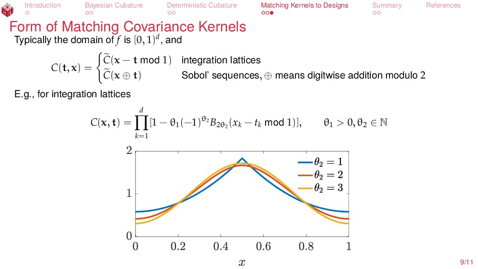
12. Introduction Bayesian Cubature Deterministic Cubature Matching Kernels to Designs Summary References Form of Matching Covariance Kernels Typically the domain of f is [0, 1)d, and C(t, x) = C(x − t mod 1) integration lattices C(x ⊕ t) Sobol’ sequences, ⊕ means digitwise addition modulo 2 E.g., for integration lattices C(x, t) = d k=1 [1 − θ1 (−1)θ2 B2θ2 (xk − tk mod 1)], θ1 > 0, θ2 ∈ N 9/11
13. Introduction Bayesian Cubature Deterministic Cubature Matching Kernels to Designs Summary References Summary Bayesian cubature leads to data-based stopping criteria There are a variety of ways to fit the covariance kernels Deterministic cubature mimics Bayesian cubature, even in the stopping rules Matching kernels to the sampling scheme makes this pratical 10/11
14. Thank you Slides available at www.slideshare.net/fjhickernell/mcqmc-2018-july-4-rennes
15. Introduction Bayesian Cubature Deterministic Cubature Matching Kernels to Designs Summary References Rathinavel, J. & H., F. J. Automatic Bayesian Cubature. in preparation. 2018+. 11/11