CalTech 2025

Talk given to the Computational and Applied Math Seminar on March 4, 2025 regarding adaptive algorithms and the importance of cones

Transcript

1. Fred J. Hickernell, Illinois Institute of Technology March 4, 2025 Adaptive Algorithms where Input Functions Lie in Cones Thanks to • Houman Owhadi and Caltech for the invitation • My collaborators • US National Science Foundation #2316011 Slides at speakerdeck.com/fjhickernell/caltech-2025
5. Next 45 minutes • Bisection method • Adaptive trapezoidal rule • Adaptive IID Monte Carlo • Adaptive quasi-Monte Carlo for cubature/expectations • Future – adaptive quasi-Monte Carlo multilevel and 
 fi nite element
6. Find such that for some with for ̂ x | ̂ x − x* | ≤ ε x* f(x* ) = 0 f ∈ 𝒞 := {f ∈ C[0,1] : f(0) f(1) ≤ 0} Bisection method Computations for this talk at https://github.com/QMCSoftware/QMCSoftware/blob/CaltechTalk2025March4/demos/ talk_paper_demos/Caltech2025March/Caltech2025MarchTalk.ipynb
7. Find such that for some with for ̂ x | ̂ x − x* | ≤ ε x* f(x* ) = 0 f ∈ 𝒞 := {f ∈ C[0,1] : f(0) f(1) ≤ 0} Bisection method Computations for this talk at https://github.com/QMCSoftware/QMCSoftware/blob/CaltechTalk2025March4/demos/ talk_paper_demos/Caltech2025March/Caltech2025MarchTalk.ipynb
8. Find such that for some with for ̂ x | ̂ x − x* | ≤ ε x* f(x* ) = 0 f ∈ 𝒞 := {f ∈ C[0,1] : f(0) f(1) ≤ 0} Bisection method Computations for this talk at https://github.com/QMCSoftware/QMCSoftware/blob/CaltechTalk2025March4/demos/ talk_paper_demos/Caltech2025March/Caltech2025MarchTalk.ipynb
9. Find such that for some with for ̂ x | ̂ x − x* | ≤ ε x* f(x* ) = 0 f ∈ 𝒞 := {f ∈ C[0,1] : f(0) f(1) ≤ 0} Bisection method Computations for this talk at https://github.com/QMCSoftware/QMCSoftware/blob/CaltechTalk2025March4/demos/ talk_paper_demos/Caltech2025March/Caltech2025MarchTalk.ipynb
10. Find such that for some with for ̂ x | ̂ x − x* | ≤ ε x* f(x* ) = 0 f ∈ 𝒞 := {f ∈ C[0,1] : f(0) f(1) ≤ 0} Bisection method Computations for this talk at https://github.com/QMCSoftware/QMCSoftware/blob/CaltechTalk2025March4/demos/ talk_paper_demos/Caltech2025March/Caltech2025MarchTalk.ipynb
11. Find such that for some with for ̂ x | ̂ x − x* | ≤ ε x* f(x* ) = 0 f ∈ 𝒞 := {f ∈ C[0,1] : f(0) f(1) ≤ 0} Bisection method Computations for this talk at https://github.com/QMCSoftware/QMCSoftware/blob/CaltechTalk2025March4/demos/ talk_paper_demos/Caltech2025March/Caltech2025MarchTalk.ipynb
12. Find such that for some with for ̂ x | ̂ x − x* | ≤ ε x* f(x* ) = 0 f ∈ 𝒞 := {f ∈ C[0,1] : f(0) f(1) ≤ 0} Bisection method Computations for this talk at https://github.com/QMCSoftware/QMCSoftware/blob/CaltechTalk2025March4/demos/ talk_paper_demos/Caltech2025March/Caltech2025MarchTalk.ipynb
13. Find such that for some with for ̂ x | ̂ x − x* | ≤ ε x* f(x* ) = 0 f ∈ 𝒞 := {f ∈ C[0,1] : f(0) f(1) ≤ 0} Bisection method Computations for this talk at https://github.com/QMCSoftware/QMCSoftware/blob/CaltechTalk2025March4/demos/ talk_paper_demos/Caltech2025March/Caltech2025MarchTalk.ipynb
14. Find such that for some with for ̂ x | ̂ x − x* | ≤ ε x* f(x* ) = 0 f ∈ 𝒞 := {f ∈ C[0,1] : f(0) f(1) ≤ 0} Bisection method Computations for this talk at https://github.com/QMCSoftware/QMCSoftware/blob/CaltechTalk2025March4/demos/ talk_paper_demos/Caltech2025March/Caltech2025MarchTalk.ipynb
15. Bisection method Finds such that for some with for is • A cone, i.e. • Non-convex, e.g., , but ̂ x | ̂ x − x* | ≤ ε x* f(x* ) = 0 f ∈ 𝒞 := {f ∈ C[0,1] : f(0) f(1) ≤ 0} 𝒞 f ∈ 𝒞 ⟹ cf ∈ 𝒞 for all c ∈ ℝ f := x ↦ x − 1/3, g := x ↦ 2/3 − x ∈ 𝒞 f/2 + g/2 = x ↦ 1/2 ∉ 𝒞
16. Trapezoidal rule ∫ 1 0 f(x) dx ≈ ?
17. Trapezoidal rule ∫ 1 0 f(x) dx ≈ n ∑ i=1 f((i − 1)/n) + f(i/n) 2n Tn (f)=∫1 0 (linear spline of f)(x) dx 0.0 0.2 0.4 0.6 0.8 1.0 x 0 1 2 3 f(x)
18. Trapezoidal rule ∫ 1 0 f(x) dx ≈ n ∑ i=1 f((i − 1)/n) + f(i/n) 2n Tn (f)=∫1 0 (linear spline of f)(x) dx 0.0 0.2 0.4 0.6 0.8 1.0 x 0 1 2 3 f(x) How big should be to make ? n errorn := ∫ 1 0 f(x) dx − Tn (f ) ≤ ε
19. Trapezoidal rule ∫ 1 0 f(x) dx ≈ n ∑ i=1 f((i − 1)/n) + f(i/n) 2n Tn (f)=∫1 0 (linear spline of f)(x) dx 0.0 0.2 0.4 0.6 0.8 1.0 x 0 1 2 3 f(x) How big should be to make ? n errorn := ∫ 1 0 f(x) dx − Tn (f ) ≤ ε Calculus says: bound ∥f′  ′  ∥
20. Trapezoidal rule ∫ 1 0 f(x) dx ≈ n ∑ i=1 f((i − 1)/n) + f(i/n) 2n Tn (f)=∫1 0 (linear spline of f)(x) dx 0.0 0.2 0.4 0.6 0.8 1.0 x 0 1 2 3 f(x) How big should be to make ? n errorn := ∫ 1 0 f(x) dx − Tn (f ) ≤ ε Calculus says: bound ∥f′  ′  ∥ easy for simple problems, hard in general
21. Trapezoidal rule ∫ 1 0 f(x) dx ≈ n ∑ i=1 f((i − 1)/n) + f(i/n) 2n Tn (f)=∫1 0 (linear spline of f)(x) dx 0.0 0.2 0.4 0.6 0.8 1.0 x 0 1 2 3 f(x) How big should be to make ? n errorn := ∫ 1 0 f(x) dx − Tn (f ) ≤ ε Calculus says: bound ∥f′  ′  ∥ Computational math says: errorn ≈ Tn − Tn/2 3 
 T12 = 1.627700615516821 = T6 ⟹ error12 ≈ 0
22. 0.0 0.2 0.4 0.6 0.8 1.0 x 0 1 2 3 f(x) Trapezoidal rule ∫ 1 0 f(x) dx ≈ n ∑ i=1 f((i − 1)/n) + f(i/n) 2n Tn (f)=∫1 0 (linear spline of f)(x) dx 0.0 0.2 0.4 0.6 0.8 1.0 x 0 1 2 3 f(x) How big should be to make ? n errorn := ∫ 1 0 f(x) dx − Tn (f ) ≤ ε Calculus says: bound ∥f′  ′  ∥ Computational math says: errorn ≈ Tn − Tn/2 3 
 T12 = 1.627700615516821 = T6 ⟹ error12 ≈ 0 Lyness [Lyn83] says, “No!” even for nice 
 f error12 = 0.0028
23. 0.0 0.2 0.4 0.6 0.8 1.0 x 0 1 2 3 f(x) 0.0 0.2 0.4 0.6 0.8 1.0 x 0 1 2 3 f(x) Trapezoidal rule errorn := ∫ 1 0 f(x) dx − n ∑ i=1 f((i − 1)/n) + f(i/n) 2n Tn ( f)=∫1 0 (linear spline of f)(x) dx ≤ Var(f′  ) 8n2
24. 0.0 0.2 0.4 0.6 0.8 1.0 x 0 1 2 3 f(x) 0.0 0.2 0.4 0.6 0.8 1.0 x 0 1 2 3 f(x) Trapezoidal rule • How big should be to make if little is known about ? n errorn ≤ ε f • Need to bound using function values Var(f′  ) = ∥f′  ′  ∥1 : ∫ 1 0 |f′  ′  (x)| dx errorn := ∫ 1 0 f(x) dx − n ∑ i=1 f((i − 1)/n) + f(i/n) 2n Tn ( f)=∫1 0 (linear spline of f)(x) dx ≤ Var(f′  ) 8n2
25. 0.0 0.2 0.4 0.6 0.8 1.0 x 0 1 2 3 f(x) 0.0 0.2 0.4 0.6 0.8 1.0 x 0 1 2 3 f(x) Trapezoidal rule • How big should be to make if little is known about ? n errorn ≤ ε f • Need to bound using function values Var(f′  ) = ∥f′  ′  ∥1 : ∫ 1 0 |f′  ′  (x)| dx 𝒞 = {f ∈ C[0,1] : Var(f′  ) ≤ fdg(1/n) Var(Sn (f )′  ) ∀n ∈ ℕ} = functions that are not too peaky where Sn (f ):= linear spline of f fdg(h):= fdg 0 (1 − h nmin )+ = fudge (in fl ation) factor errorn := ∫ 1 0 f(x) dx − n ∑ i=1 f((i − 1)/n) + f(i/n) 2n Tn ( f)=∫1 0 (linear spline of f)(x) dx ≤ Var(f′  ) 8n2
26. 1. Given and tolerance, , choose . 2. Compute 3. While , double and go to step 2 4. Return guaranteed to make if At a computational cost function values fdg(h) := fdg0 (1 − h nmin )+ ε n = 2nmin errorn := fdg(1/n) Var(Sn (f )′  ) 8n2 errorn > ε n Tn (f ) errorn ≤ errorn ≤ ε f ∈ ≤ 1 + 2nmin + fdg0 Var(f′  ) 2ε Adaptive sample size trapezoidal rule errorn := ∫ 1 0 f(x) dx − n ∑ i=1 f((i − 1)/n) + f(i/n) 2n Tn ( f) ≤ Var(f′  ) 8n2
27. 1. Given and tolerance, , choose . 2. Compute 3. While , double and go to step 2 4. Return guaranteed to make if At a computational cost function values fdg(h) := fdg0 (1 − h nmin )+ ε n = 2nmin errorn := fdg(1/n) Var(Sn (f )′  ) 8n2 errorn > ε n Tn (f ) errorn ≤ errorn ≤ ε f ∈ ≤ 1 + 2nmin + fdg0 Var(f′  ) 2ε Adaptive sample size trapezoidal rule errorn := ∫ 1 0 f(x) dx − n ∑ i=1 f((i − 1)/n) + f(i/n) 2n Tn ( f) ≤ Var(f′  ) 8n2
28. Observations
29. • Computational cost is without knowing a priori 𝒪 ( Var(f′  )/ε) Var(f′  ) Observations
30. • Computational cost is without knowing a priori 𝒪 ( Var(f′  )/ε) Var(f′  ) • Typically, cannot know whether black box is inside
 but f ‣ The cone de fi nes nice functions precisely Observations
31. • Computational cost is without knowing a priori 𝒪 ( Var(f′  )/ε) Var(f′  ) • Typically, cannot know whether black box is inside
 but f ‣ The cone de fi nes nice functions precisely ‣ You cannot know whether is inside either f Observations
32. • Computational cost is without knowing a priori 𝒪 ( Var(f′  )/ε) Var(f′  ) • Typically, cannot know whether black box is inside
 but f ‣ The cone de fi nes nice functions precisely ‣ You cannot know whether is inside either f • Bakhvalov [Bak70] proved that adaptive algorithms for linear problems de fi ned on convex, balanced sets of input functions cannot do signi fi cantly better than non-adaptive algorithms Observations
33. 𝒞 := {f ∈ C[0,1] : Var(f′  , [β, γ]) ≤ ˜ V (f, α, β, γ, δ) ∀α < β < γ < δ} ˜ V (f, α, β, γ, δ) := max(fdg(γ − α) Var(S(f, α, β, γ)′  ), fdg(δ − β) Var(S(f, β, γ, δ)′  ) 0 ≤ α < β < γ < δ ≤ 1, fdg(γ − α) Var(S(f, α, β, γ)′  ) 0 ≤ α < β < γ ≤ 1 < δ fdg(δ − β) Var(S(f, β, γ, δ)′  ) α < 0 ≤ β < γ < δ ≤ 1 error({xi }n i=0 ):= n ∑ i=1 errori where errori := ˜ V (f, xi−2 , xi−1 , xi , xi+1 )(xi − xi−1 )2 8 Adaptive node placement trapezoidal rule errorn := ∫ 1 0 f(x) dx − n ∑ i=1 f(xi−1 ) + f(xi ) 2 (xi − xi−1 ) T(f;{xi }n−1 i=0 )=∫1 0 (linear spline of f)(x) dx ≤ n ∑ i=1 Var(f′  , [xi−1 , xi ]) (xi − xi−1 )2 8
34. 1. Given and tolerance, , choose . 2. Compute 3. While , subdivide with largest and go to step 2 4. Return guaranteed to make if At a computational cost but with a smaller constant, 
 see [CDHT17] fdg( ⋅ ) ε n = 3nmin error({xi }n i=0 ) := n ∑ i=1 errori , errori := ˜ V (f, xi−2 , xi−1 , xi , xi+1 ) 8(xi − xi−1 )2 error({xi }n i=0 ) > ε [xi−1 , xi ] errori T(f; {xi }n i=0 ) error({xi }n i=0 ) ≤ error({xi }n i=0 ) ≤ ε f ∈ 𝒪 (ε−1/2) Adaptive node placement trapezoidal rule errorn := ∫ 1 0 f(x) dx − n ∑ i=1 f(xi−1 ) + f(xi ) 2(xi − xi−1 ) T(f;{xi }n−1 i=0 )=∫1 0 (linear spline of f)(x) dx ≤ n ∑ i=1 Var(f′  , [xi−1 , xi ]) (xi − xi−1 )2 8
35. 1. Given and tolerance, , choose . 2. Compute 3. While , subdivide with largest and go to step 2 4. Return guaranteed to make if At a computational cost but with a smaller constant, 
 see [CDHT17] fdg( ⋅ ) ε n = 3nmin error({xi }n i=0 ) := n ∑ i=1 errori , errori := ˜ V (f, xi−2 , xi−1 , xi , xi+1 ) 8(xi − xi−1 )2 error({xi }n i=0 ) > ε [xi−1 , xi ] errori T(f; {xi }n i=0 ) error({xi }n i=0 ) ≤ error({xi }n i=0 ) ≤ ε f ∈ 𝒪 (ε−1/2) Adaptive node placement trapezoidal rule errorn := ∫ 1 0 f(x) dx − n ∑ i=1 f(xi−1 ) + f(xi ) 2(xi − xi−1 ) T(f;{xi }n−1 i=0 )=∫1 0 (linear spline of f)(x) dx ≤ n ∑ i=1 Var(f′  , [xi−1 , xi ]) (xi − xi−1 )2 8
36. Adaptive sample size vs. node placement 0.0 0.2 0.4 0.6 0.8 1.0 x 0 2 4 6 8 10 12 f(x) 70 Trapezoids 0.0 0.2 0.4 0.6 0.8 1.0 x 0 2 4 6 8 10 12 f(x) 320 Trapezoids 10°8 10°7 10°6 10°5 10°4 10°3 10°2 Error tolerance, " 102 103 104 105 # of trapezoids, n adaptive n adaptive xi p Var(f0)/(8") 2nmin + p fdg0 Var(f0)/(2") ε = 0.005
37. Does this remind us of something statistical?
38. • Trapezoidal rule approximates from and by bounding ∫ 1 0 f(x) dx {f(xi )}n i=1 Var(f′  ) Does this remind us of something statistical?
39. • Trapezoidal rule approximates from and by bounding ∫ 1 0 f(x) dx {f(xi )}n i=1 Var(f′  ) • Monte Carlo approximates by , for μ := ∫ [0,1]d f(x) dx ̂ μn := 1 n n ∑ i=1 f(xi ) {xi }n i=1 IID ∼ 𝒰 [0,1]d Does this remind us of something statistical?
40. • Trapezoidal rule approximates from and by bounding ∫ 1 0 f(x) dx {f(xi )}n i=1 Var(f′  ) • Monte Carlo approximates by , for μ := ∫ [0,1]d f(x) dx ̂ μn := 1 n n ∑ i=1 f(xi ) {xi }n i=1 IID ∼ 𝒰 [0,1]d ‣ Chebyshev’s Inequality: for ℙ[|μ − ̂ μn | ≤ 5σ/ n] ≥ 96 % f ∈ {f : Std(f ) ≤ σ} Does this remind us of something statistical?
41. • Trapezoidal rule approximates from and by bounding ∫ 1 0 f(x) dx {f(xi )}n i=1 Var(f′  ) • Monte Carlo approximates by , for μ := ∫ [0,1]d f(x) dx ̂ μn := 1 n n ∑ i=1 f(xi ) {xi }n i=1 IID ∼ 𝒰 [0,1]d ‣ Chebyshev’s Inequality: for ℙ[|μ − ̂ μn | ≤ 5σ/ n] ≥ 96 % f ∈ {f : Std(f ) ≤ σ} Does this remind us of something statistical?
42. • Trapezoidal rule approximates from and by bounding ∫ 1 0 f(x) dx {f(xi )}n i=1 Var(f′  ) • Monte Carlo approximates by , for μ := ∫ [0,1]d f(x) dx ̂ μn := 1 n n ∑ i=1 f(xi ) {xi }n i=1 IID ∼ 𝒰 [0,1]d ‣ Chebyshev’s Inequality: for ℙ[|μ − ̂ μn | ≤ 5σ/ n] ≥ 96 % f ∈ {f : Std(f ) ≤ σ} ‣ Central Limit Theorem: Compute the sample standard deviation, , 
 for of nice functions
 [HJLO13] gives a rigorous approach 
 using Berry-Esseen inequalities ̂ σ ℙ[ |μ − ̂ μn | ≤ 1.96 fdg(n) ̂ σ / n ] ≥ 95 % f ∈ • Bahadur and Savage [BS56] explain why the cone should be non-convex Does this remind us of something statistical?
43. Multi- integrals/expectations in practice d μ := expectation 𝔼 [f( X ⏟ ∼ 𝒰 [0,1]d ) = integral ∫ [0,1]d f(x) dx ≈ sample mean 1 n n ∑ i=1 f(xi ) =: ̂ μn f(X) = option payo ff underground water pressure with random rock porosity pixel intensity from random ray option price average water pressure average pixel intensity = μ may be dozens or hundreds d
44. Low discrepancy (LD) sequences can beat grids and IID for moderate to large d Quasi-Monte Carlo (QMC) methods [HKS25] 0.00 0.25 0.50 0.75 1.00 xi1 0.00 0.25 0.50 0.75 1.00 xi2 64 IID points for d = 6 0.0 0.2 0.4 0.6 0.8 1.0 xi1 0.0 0.2 0.4 0.6 0.8 1.0 xi2 64 Grid Points for d =6 0.00 0.25 0.50 0.75 1.00 xi1 0.00 0.25 0.50 0.75 1.00 xi2 64 Sobol’ points for d = 6 0.00 0.25 0.50 0.75 1.00 xi1 0.00 0.25 0.50 0.75 1.00 xi2 64 Lattice Points for d = 6
45. Low discrepancy (LD) sequences can beat grids and IID for moderate to large d Quasi-Monte Carlo methods 100 101 102 103 104 105 106 107 Sample Size, n 10°6 10°4 10°2 100 Relative Error, |(µ ° ˆ µn )/µ| grid O(n°1/5) IID MC med O(n°1/2) LD med O(n°1) μ = ∫ ℝ6 cos(∥x∥) exp( −∥x∥2) dx [Kei96]
46. Discrepancy measures the quality of [H00] x0 , x1 , … μ := expectation 𝔼 [f( X ⏟ ∼ 𝒰 ([0,1]d) )] = integral ∫ [0,1]d f(x) dx ≈ sample mean 1 n n ∑ i=1 f(xi ) =: ̂ μn |μ − ̂ μn | ≤ tight discrepancy({xi }n i=1 ) norm of the error functional variation(f ) semi-norm
47. Discrepancy measures the quality of [H00] x0 , x1 , … μ := expectation 𝔼 [f( X ⏟ ∼ 𝒰 ([0,1]d) )] = integral ∫ [0,1]d f(x) dx ≈ sample mean 1 n n ∑ i=1 f(xi ) =: ̂ μn |μ − ̂ μn | ≤ tight discrepancy({xi }n i=1 ) norm of the error functional variation(f ) semi-norm If is in a Hilbert space with reproducing kernel , then f ℋ K discrepancy2({xi }n i=1 ) = ∫ [0,1]d×[0,1]d K(t, x) dt dx − 2 n n ∑ i=1 ∫ [0,1]d K(t, xi ) dt + 1 n2 n ∑ i,j=1 K(xi , xj ) variation(f ) = inf c∈ℝ ∥f − c∥ℋ
48. Discrepancy measures the quality of [H00] x0 , x1 , … μ := expectation 𝔼 [f( X ⏟ ∼ 𝒰 ([0,1]d) )] = integral ∫ [0,1]d f(x) dx ≈ sample mean 1 n n ∑ i=1 f(xi ) =: ̂ μn |μ − ̂ μn | ≤ tight discrepancy({xi }n i=1 ) norm of the error functional variation(f ) semi-norm If is in a Hilbert space with reproducing kernel , then f ℋ K discrepancy2({xi }n i=1 ) = ∫ [0,1]d×[0,1]d K(t, x) dt dx − 2 n n ∑ i=1 ∫ [0,1]d K(t, xi ) dt + 1 n2 n ∑ i,j=1 K(xi , xj ) variation(f ) = inf c∈ℝ ∥f − c∥ℋ operations 𝒪 (dn2) infeasible to compute
49. Deterministic stopping rules for QMC [HJ16, JH16, SJ24] μ := expectation 𝔼 [f( X ⏟ ∼ 𝒰 ([0,1]d) )] = integral ∫ [0,1]d f(x) dx ≈ sample mean 1 n n ∑ i=1 f(xi ) =: ̂ μn , want |μ − ̂ μn | ≤ ε
50. Deterministic stopping rules for QMC [HJ16, JH16, SJ24] μ := expectation 𝔼 [f( X ⏟ ∼ 𝒰 ([0,1]d) )] = integral ∫ [0,1]d f(x) dx ≈ sample mean 1 n n ∑ i=1 f(xi ) =: ̂ μn , want |μ − ̂ μn | ≤ ε • For lattices, , , ̂ f(k) := ∫ [0,1]d f(x) 𝖾 −2π −1kT x dx f(x) = ∑ k∈ℤd ̂ f(k) 𝖾 2π −1kT x μ = ̂ f(0)
51. Deterministic stopping rules for QMC [HJ16, JH16, SJ24] μ := expectation 𝔼 [f( X ⏟ ∼ 𝒰 ([0,1]d) )] = integral ∫ [0,1]d f(x) dx ≈ sample mean 1 n n ∑ i=1 f(xi ) =: ̂ μn , want |μ − ̂ μn | ≤ ε • For lattices, , , ̂ f(k) := ∫ [0,1]d f(x) 𝖾 −2π −1kT x dx f(x) = ∑ k∈ℤd ̂ f(k) 𝖾 2π −1kT x μ = ̂ f(0) • due to aliasing ( constant for all ) μ − ̂ μn 𝖾 2π −1kT xi i
52. Deterministic stopping rules for QMC [HJ16, JH16, SJ24] μ := expectation 𝔼 [f( X ⏟ ∼ 𝒰 ([0,1]d) )] = integral ∫ [0,1]d f(x) dx ≈ sample mean 1 n n ∑ i=1 f(xi ) =: ̂ μn , want |μ − ̂ μn | ≤ ε • For lattices, , , ̂ f(k) := ∫ [0,1]d f(x) 𝖾 −2π −1kT x dx f(x) = ∑ k∈ℤd ̂ f(k) 𝖾 2π −1kT x μ = ̂ f(0) • due to aliasing ( constant for all ) μ − ̂ μn 𝖾 2π −1kT xi i • Assume that lies in of functions whose Fourier coe ffi cients decay reasonably f
53. Deterministic stopping rules for QMC [HJ16, JH16, SJ24] μ := expectation 𝔼 [f( X ⏟ ∼ 𝒰 ([0,1]d) )] = integral ∫ [0,1]d f(x) dx ≈ sample mean 1 n n ∑ i=1 f(xi ) =: ̂ μn , want |μ − ̂ μn | ≤ ε • For lattices, , , ̂ f(k) := ∫ [0,1]d f(x) 𝖾 −2π −1kT x dx f(x) = ∑ k∈ℤd ̂ f(k) 𝖾 2π −1kT x μ = ̂ f(0) • due to aliasing ( constant for all ) μ − ̂ μn 𝖾 2π −1kT xi i • Assume that lies in of functions whose Fourier coe ffi cients decay reasonably f • Approximate by a one-dimensional FFT of ̂ f(k) {f(xi )}n−1 i=0
54. Deterministic stopping rules for QMC [HJ16, JH16, SJ24] μ := expectation 𝔼 [f( X ⏟ ∼ 𝒰 ([0,1]d) )] = integral ∫ [0,1]d f(x) dx ≈ sample mean 1 n n ∑ i=1 f(xi ) =: ̂ μn , want |μ − ̂ μn | ≤ ε • For lattices, , , ̂ f(k) := ∫ [0,1]d f(x) 𝖾 −2π −1kT x dx f(x) = ∑ k∈ℤd ̂ f(k) 𝖾 2π −1kT x μ = ̂ f(0) • due to aliasing ( constant for all ) μ − ̂ μn 𝖾 2π −1kT xi i • Assume that lies in of functions whose Fourier coe ffi cients decay reasonably f • Approximate by a one-dimensional FFT of ̂ f(k) {f(xi )}n−1 i=0 • FFT approximations provide a rigorous data-driven bound on with work μ − ̂ μn 𝒪 (n log n)
55. Deterministic stopping rules for QMC [HJ16, JH16, SJ24] μ := expectation 𝔼 [f( X ⏟ ∼ 𝒰 ([0,1]d) )] = integral ∫ [0,1]d f(x) dx ≈ sample mean 1 n n ∑ i=1 f(xi ) =: ̂ μn , want |μ − ̂ μn | ≤ ε • For lattices, , , ̂ f(k) := ∫ [0,1]d f(x) 𝖾 −2π −1kT x dx f(x) = ∑ k∈ℤd ̂ f(k) 𝖾 2π −1kT x μ = ̂ f(0) • due to aliasing ( constant for all ) μ − ̂ μn 𝖾 2π −1kT xi i • Assume that lies in of functions whose Fourier coe ffi cients decay reasonably f • Approximate by a one-dimensional FFT of ̂ f(k) {f(xi )}n−1 i=0 • FFT approximations provide a rigorous data-driven bound on with work μ − ̂ μn 𝒪 (n log n) • Similarly for digital nets
56. Bayesian stopping rules for QMC [JH19, JH22] μ := expectation 𝔼 [f( X ⏟ ∼ 𝒰 ([0,1]d) )] = integral ∫ [0,1]d f(x) dx ≈ sample mean 1 n n ∑ i=1 f(xi ) =: ̂ μn , want |μ − ̂ μn | ≤ ε • Assume is a Gaussian stochastic process with covariance kernel , where the hyper-parameters are properly tuned, • Construct a Bayesian credible interval for • If is chosen to fi t the lattice/digital sequences, then the computation normally required reduces to • Works for in f K μ K 𝒪 (n3) 𝒪 (n log n) f For an alternative view, see [LENOT24]
57. Keister example sample size and time μ = ∫ ℝ6 cos(∥x∥) exp( −∥x∥2) dx [Kei96] 10°4 10°3 10°2 10°1 Relative error tolerance, " 102 103 104 105 106 107 Sample size, n Sobol’ deterministic lattice deterministic Sobol’ Bayesian lattice Bayesian 10°4 10°3 10°2 10°1 Relative error tolerance, " 10°4 10°3 10°2 10°1 100 101 Computation time (sec) Sobol’ deterministic lattice deterministic Sobol’ Bayesian lattice Bayesian
58. What comes next for rigorous adaptive methods? Adaptive 1-D Integration Adaptive (quasi-)Monte Carlo
59. What comes next for rigorous adaptive methods? Adaptive 1-D Integration Adaptive (quasi-)Monte Carlo Adaptive multi-level (quasi-)Monte Carlo
60. What comes next for rigorous adaptive methods? Adaptive 1-D Integration Adaptive (quasi-)Monte Carlo Adaptive multi-level (quasi-)Monte Carlo Adaptive FEM for PDEs w/ a posteriori error bounds
61. What comes next for rigorous adaptive methods? Adaptive 1-D Integration Adaptive (quasi-)Monte Carlo Adaptive multi-level (quasi-)Monte Carlo Adaptive FEM for PDEs w/ a posteriori error bounds Adaptive multi-level (quasi-)Monte Carlo with FEM for PDEs with randomness
62. Past 50 minutes • Ice cream cones • Bisection method • Adaptive trapezoidal rule • Adaptive IID Monte Carlo • Adaptive quasi-Monte Carlo for cubature/expectations • Future work – adaptive multilevel and fi nite element • May we talk?
63. MCM2025Chicago.org July 28 – August 1 Plenary Speakers Nicholas Chopin, ENSAE Peter Glynn, Stanford U
 Roshan Joseph, Georgia Tech Christiane Lemieux, U Waterloo
 Matt Pharr, NVIDIA Veronika Rockova, U Chicago
 Uros Seljak, U California, Berkeley Michaela Szölgyenyi, U Klagenfurt
64. References [Bak70] N. S. Bakhvalov, On the optimality of linear methods for operator approximation in convex classes of functions (in Russian), Zh. Vychisl. Mat. i Mat. Fiz. 10 (1970), 555–568, English transl.: USSR Comput. Math. Math. Phys. 11 (1971) 244–249. [BS56] R. R. Bahadur and L. J. Savage, The nonexistence of certain statistical procedures in nonparametric problems, Ann. Math. Stat. 27 (1956), 1115–1122. [CDHT17] S. C. T. Choi, Y. Ding, F. J. Hickernell, and X. Tong, Local adaption for approximation and minimization of univariate functions, J. Complexity {40} (2017), 17–33. [Gil15] M. B. Giles, Multilevel Monte Carlo methods, Acta Numer. 24 (2015), 259–328. [H00] F. J. Hickernell, What a ff ects the accuracy of quasi-Monte Carlo quadrature?, Monte Carlo and Quasi-Monte Carlo Methods 1998 (H. Niederreiter and J. Spanier, eds.), Springer-Verlag, Berlin, 2000, pp. 16–55.
65. References [HJLO13] F. J. Hickernell, L. Jiang, Y. Liu, and A. B. Owen, Guaranteed conservative fi xed width con fi dence intervals via Monte Carlo sampling, Monte Carlo and Quasi-{M}onte {C}arlo Methods 2012 (J. Dick, F. Y. Kuo, G. W. Peters, and I. H. Sloan, eds.), Springer Proceedings in Mathematics and Statistics, vol. 65, Springer-Verlag, Berlin, 2013, pp. 105–128.[ [HJ16] F. J. Hickernell and Ll. A. Jiménez Rugama, Reliable adaptive cubature using digital sequences, Monte Carlo and Quasi-Monte Carlo Methods: MCQMC, Leuven, Belgium, April 2014 (R. Cools and D. Nuyens, eds.), Springer Proceedings in Mathematics and Statistics, vol. 163, Springer-Verlag, Berlin, 2016, pp. 367–383. [HJLO13] F. J. Hickernell, L. Jiang, Y. Liu, and A. B. Owen, Guaranteed conservative fi xed width con fi dence intervals via Monte Carlo sampling, Monte Carlo and Quasi-Monte Carlo Methods 2012 (J. Dick, F. Y. Kuo, G. W. Peters, and I. H. Sloan, eds.), Springer Proceedings in Mathematics and Statistics, vol. 65, Springer-Verlag, Berlin, 2013, pp. 105–128. [HKS25] F. J. Hickernell, N. Kirk, and A. G. Sorokin, Quasi-Monte Carlo methods: What, why, and how?, submitted to MCQMC 2024 proceedings, https://doi.org/10.48550/arXiv.2502.03644, 2025+.
66. References [JH19] R. Jagadeeswaran and F. J. Hickernell, Fast automatic Bayesian cubature using lattice sampling, Stat. Comput. 29 (2019), 1215–1229. [JH22] R. Jagadeeswaran and F. J. Hickernell, Fast automatic Bayesian cubature using Sobol' sampling, Advances in Modeling and Simulation: Festschrift in Honour of Pierre L'Ecuyer (Z. Botev, A. Keller, C. Lemieux, and B. Tu ff i n, eds.), Springer, Cham, 2022, pp. 301–318. [JH16] Ll. A. Jiménez Rugama and F. J. Hickernell, Adaptive multidimensional integration based on rank-1 lattices, Monte Carlo and Quasi-Monte Carlo Methods: MCQMC, Leuven, Belgium, April 2014 (R. Cools and D. Nuyens, eds.), Springer Proceedings in Mathematics and Statistics, vol. 163, Springer-Verlag, Berlin, 2016, pp. 407–422. 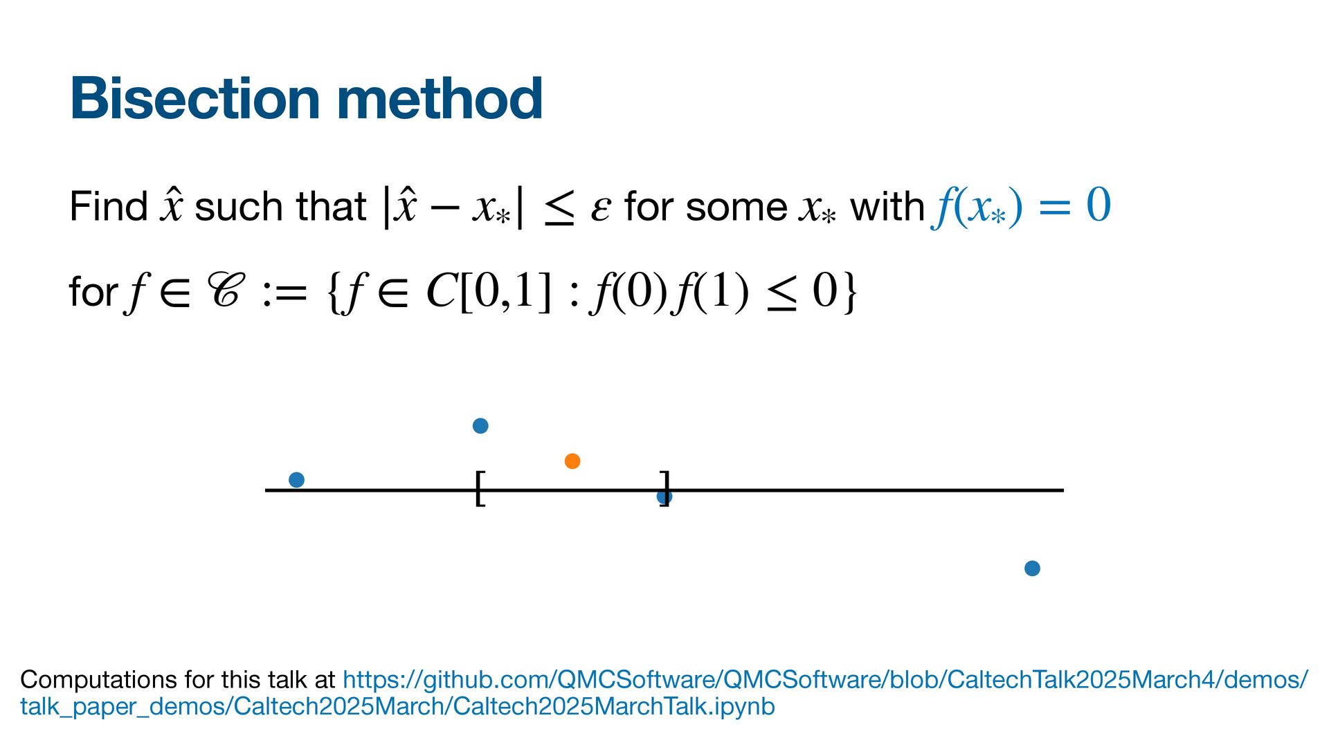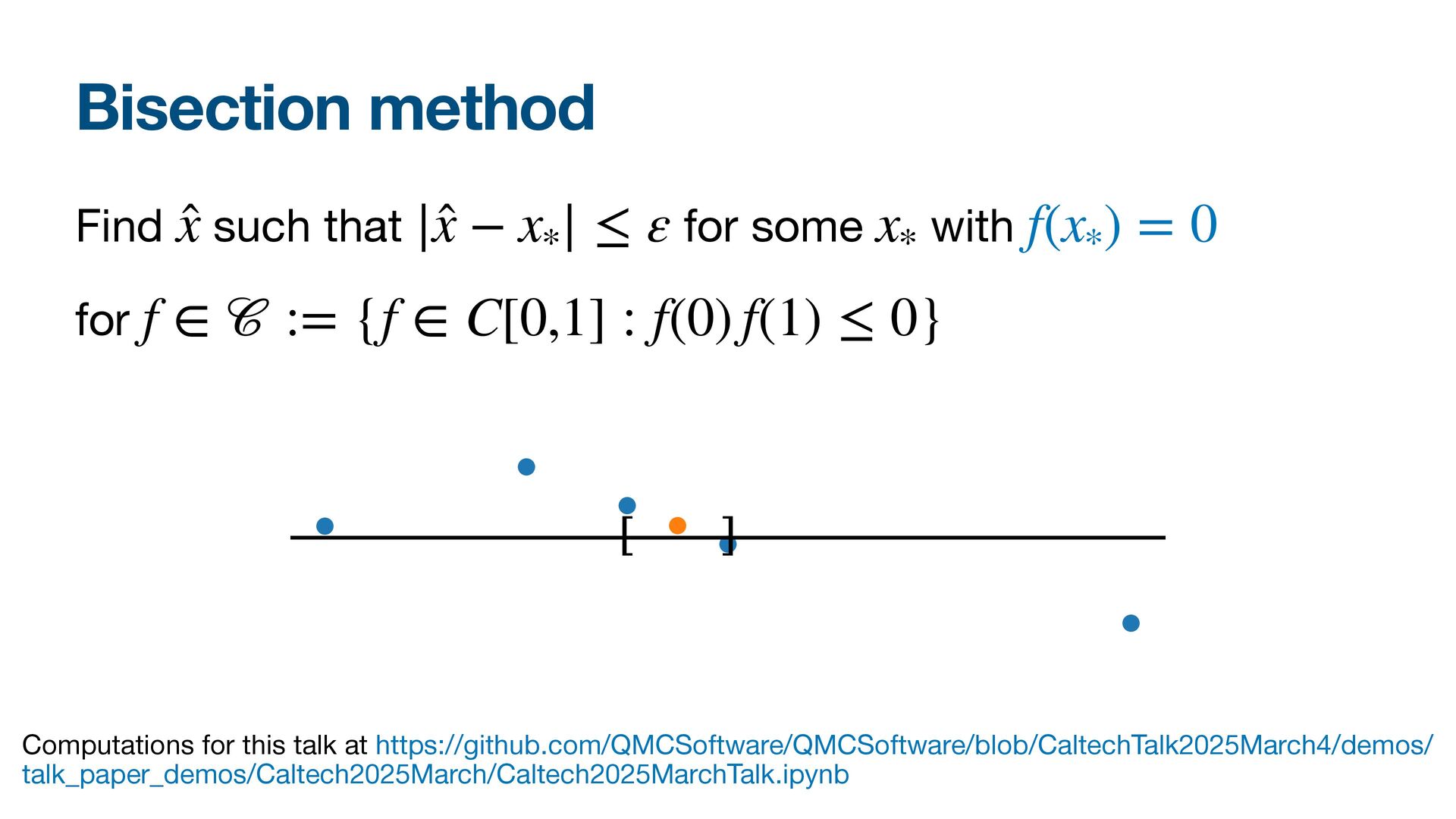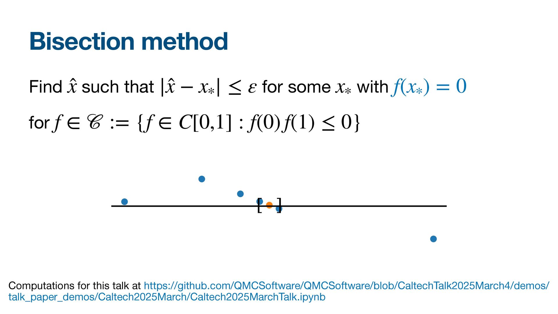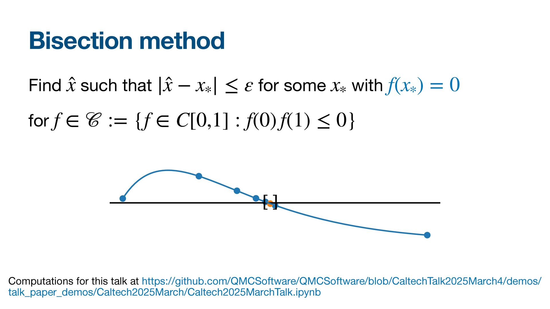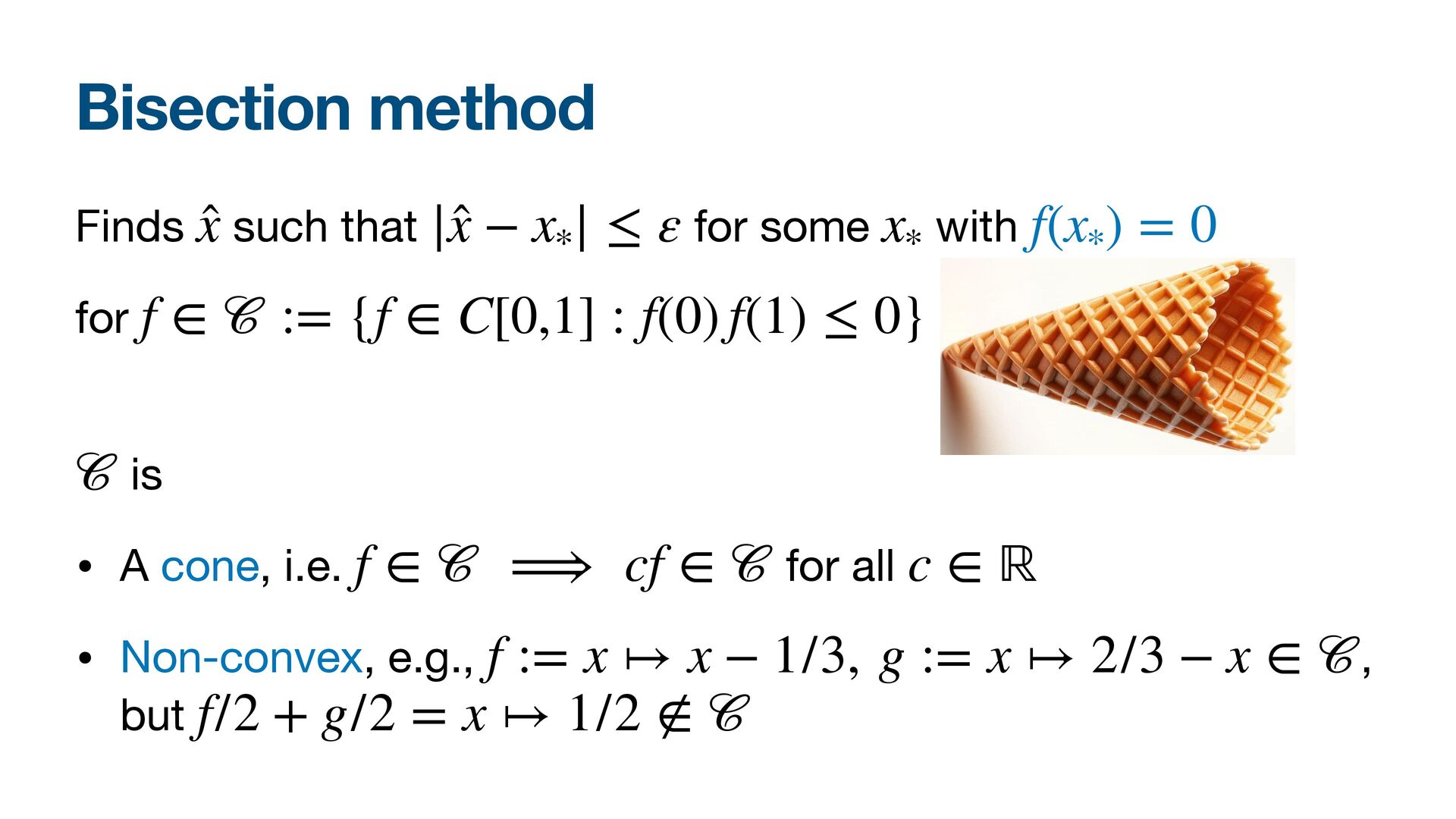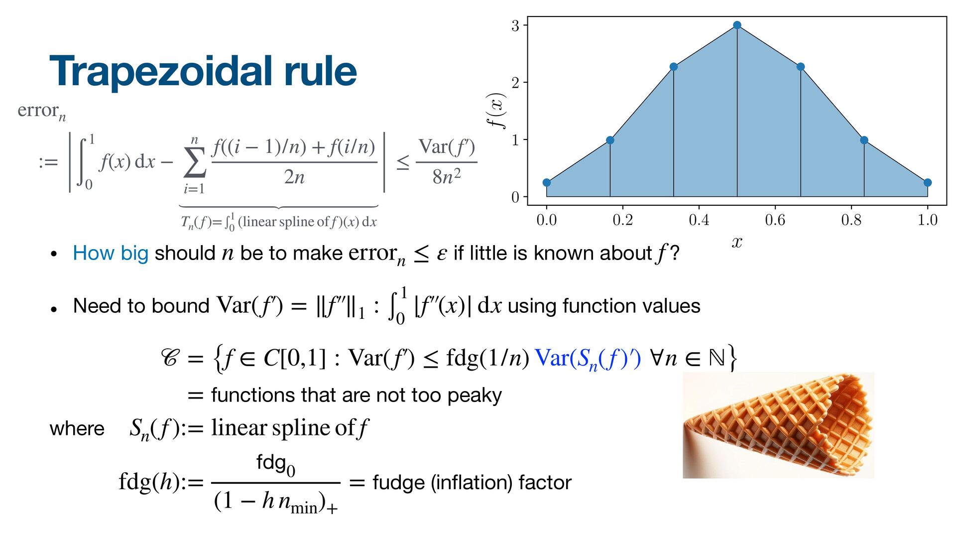[Kei96] B. D. Keister, Multidimensional quadrature algorithms, Computers in Physics 10 (1996), 119– 122. [LENOT24] P. L'Ecuyer, M. K. Nakayama, A. B. Owen, and B. Tu ffi n, Con fi dence intervals for randomized quasi-Monte Carlo estimators, WSC ’23: Proceedings of the Winter Simulation Conference, 2024, pp. 445–456.
67. References [Lyn83] J. N. Lyness, When not to use an automatic quadrature routine, SIAM Rev. 25 (1983), 63–87. [SJ24] A. G. Sorokin and R. Jagadeeswaran, On bounding and approximating functions of multiple expectations using quasi-Monte Carlo, Monte Carlo and Quasi-Monte Carlo Methods: MCQMC, Linz, Austria, July 2022 (A. Hinrichs, P. Kritzer, and F. Pillichshammer, eds.), Springer Proceedings in Mathematics and Statistics, Springer, Cham, 2024, pp. 583–589.
68. Multilevel methods reduce computational cost [Gil15] μ := expectation 𝔼 [f( X ⏟ ∼ 𝒰 ([0,1]d) )] = integral ∫ [0,1]d f(x) dx ≈ sample mean 1 n n ∑ i=1 f(xi ) =: ̂ μn • The cost to evaluate is typically , so the cost to obtain is typically • If one can approximate by lower dimensional approximations, , then f(xi ) 𝒪 (d) |μ − ̂ μn | ≤ ε 𝒪 (dε−1−δ) f fs : [0,1]s → ℝ • Balance the cost to approximate well and the total cost to obtain may be as small as as 𝒪 (nl sl ) μ(s) |μ − ̂ μn | ≤ ε 𝒪 (ε−1−δ) d, ε−1 → ∞
69. Multilevel methods reduce computational cost [Gil15] μ := expectation 𝔼 [f( X ⏟ ∼ 𝒰 ([0,1]d) )] = integral ∫ [0,1]d f(x) dx ≈ sample mean 1 n n ∑ i=1 f(xi ) =: ̂ μn • The cost to evaluate is typically , so the cost to obtain is typically • If one can approximate by lower dimensional approximations, , then f(xi ) 𝒪 (d) |μ − ̂ μn | ≤ ε 𝒪 (dε−1−δ) f fs : [0,1]s → ℝ μ = 𝔼 [fs1 (X1:s1 )] μ(1) + 𝔼 [fs2 (X1:s2 ) − fs1 (X1:s1 )] μ(2) + ⋯ + 𝔼 [f(X1:d ) − fsL−1 (X1:sL−1 )] μ(L) • Balance the cost to approximate well and the total cost to obtain may be as small as as 𝒪 (nl sl ) μ(s) |μ − ̂ μn | ≤ ε 𝒪 (ε−1−δ) d, ε−1 → ∞