SunPy: Python for solar physics

Transcript

1. Steven Christe1,, Matt Earnshaw2, Keith Hughitt1, Jack Ireland1, Florian Mayer3, Albert Shih1, Alex Young1 1 NASA GSFC 2 Imperial College London 3 Vienna University of Technology Florian Mayer
2.  What is Python?  Introduction to Python  Scientific Python  NumPy  Matplotlib  SciPy  Python in solar physics
3.  General-purpose  Object-oriented (disputed)  Cross-platform  Windows  Mac OS  Linux  Other Unices (FreeBSD, Solaris, etc.)  High-level
4.  Internet companies  Google  Rackspace  Games  Battlefield 2  Civilization 4  Graphics  Walt Disney  Science  NASA  ESRI
5.  Easy  Comprehensive standard library (“batteries included”) Quality does vary, though.  Good support for scientific tasks  Permissive open-source license On the downside:  Slower, but ways to speed up
6. PYTHON IDL  Proprietary software  License cost  Small community  Cumbersome plotting  Solar software  Free open-source software  Without cost  General purpose  Good plotting  No solar software
7.  Implementation started 1989 by Guido van Rossum (BDFL)  2.0 appeared 2000  Garbage collection  Unicode  3.0 appeared 2008
8.  Astronomy  Artificial intelligence & machine learning  Bayesian Statistics  Biology (including Neuroscience)  Dynamical systems  Economics and Econometrics  Electromagnetics  Electrical Engineering  Geosciences  Molecular modeling  Signal processing  Symbolic math, number theory
9.  pyFITS – read FITS files  pyRAF – run IRAF tasks  pywcs  pyephem – compute positions of objects in space  spacepy (space sciences, just released)  Planned standard library AstroPy
10.  Beautiful is better than ugly.  Explicit is better than implicit.  Simple is better than complex.  Readability counts.  There should be one – and preferably only one – obvious way to do it.  Although that way may not be obvious at first unless you're Dutch.  >>> import this
11. Brief introduction into Python
12.  Infix notation operations  Python 2 defaults to floor division  More mathematical operations in math  Complex math in cmath
13.  Integers are arbitrary size.  Floats are platform doubles.  decimal module for arbitrary precision decimal numbers  fractions module for fractions
14. STRINGS / BYTES  "foo"  Store bytes  Useful for binary data UNICODE  u"foo"  Store unicode codepoints  Useful for text  Behave as expected for multibyte characters
15.  [1, 2, 3, 4]  Mutable  Multiple records  (1, u"foo")  Immutable  Different objects describing one record
16.  if/elif/else  for-loop  break  continue  else  while-loop  pass
17.  Default arguments are evaluated once at compile time!  lambda alternative syntax for definition of trivial functions  Functions are objects, too!
18.  Unordered key-value mappings  Approx. O(1) lookup and storage  Keys must be immutable (hashable)
19.  Unordered collection of unique objects  Approx. O(1) membership test  Members must be immutable (hashable)
20.  Classes  Explicit self  Multiple inheritance  Also in IDL 8; no escaping it
21.  try / except / else  raise  Exceptions inherit from Exception
22. PYTHON 2.7  Print statement  String / Unicode  Floor division  Relative imports  Lists PYTHON 3.2  Print function  Bytes / String  Float Division  Absolute imports  Views Tons of other changes http://bit.ly/newpy3
23.  Fundamental package for science in Python  Multidimensional fixed-size, homogenous arrays  Derived objects: e.g. matrices  More efficient  Less code
24.  Python list  arange  linspace / logspace  ones / zeros / eye / diag  random
25.  Absence of explicit looping  Conciseness – less bugs  Closer to mathematical notation  More pythonic.  Also possible for user functions
26.  Expansion of multidimensional arrays  Implicit element-by-element behavior
33.  Boolean area  Integer area
34. Type Remarks Character code byte compatible: C char 'b' short compatible: C short 'h' intc compatible: C int 'i' int_ compatible: Python int 'l' longlong compatible: C long long 'q' intp large enough to fit a pointer 'p' int8 8 bits int16 16 bits int32 32 bits int64 64 bits
35. Type Remarks Character code ubyte compatible: C u. char 'B' ushort compatible: C u. short 'H' uintc compatible: C unsigned int 'I' uint compatible: Python int 'L' ulonglong compatible: C long long 'Q' uintp large enough to fit a pointer 'P' uint8 8 bits uint16 16 bits uint32 32 bits uint64 64 bits
36. Type Remarks Character code half 'e' single compatible: C float 'f' double compatible: C double float_ compatible: Python float 'd' longfloat compatible: C long float 'g' float16 16 bits float32 32 bits float64 64 bits float96 96 bits, platform? float128 128 bits, platform?
37. Type Remarks Character code csingle 'F' complex_ compatible: Python complex 'D' clongfloat 'G' complex64 two 32-bit floats complex128 two 64-bit floats complex192 two 96-bit floats, platform? complex256 two 128-bit floats, platform?
38.  NumPy: weave.blitz (fast NumPy expressions)  NumPy: weave.inline (inline C/C++)  f2py (interface Fortran)  Pyrex/Cython (python-like compiled language)
39.  2D plotting library  Some 3D support  Publication-quality figures  “Make easy things easy and hard things possible”  Configurable using matplotlibrc
40. import numpy as np from matplotlib import pyplot as plt t = np.linspace(0, 2, 200) s = np.sin(2*pi*t) plt.plot(t, s, linewidth=1.0) plt.xlabel('time (s)') plt.ylabel('voltage (mV)') plt.title('About as simple as it gets, folks') plt.grid(True) plt.show()
41. import numpy as np from matplotlib import pyplot as plt def f(t): s1 = np.cos(2*pi*t) e1 = np.exp(-t) return np.multiply(s1,e1) t1 = np.arange(0.0, 5.0, 0.1) t2 = np.arange(0.0, 5.0, 0.02) t3 = np.arange(0.0, 2.0, 0.01) plt.subplot(211) l = plot(t1, f(t1), 'bo', t2, f(t2), 'k--', markerfacecolor='green') plt.grid(True) plt.title('A tale of 2 subplots') plt.ylabel('Damped oscillation') plt.subplot(212) plt.plot(t3, np.cos(2*pi*t3), 'r.') plt.grid(True) plt.xlabel('time (s)') plt.ylabel('Undamped') plt.show()
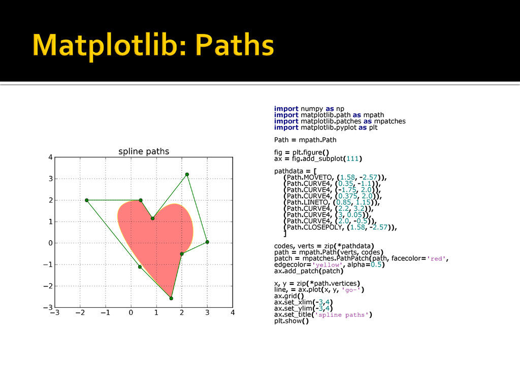
42. import numpy as np import matplotlib.path as mpath import matplotlib.patches as mpatches import matplotlib.pyplot as plt Path = mpath.Path fig = plt.figure() ax = fig.add_subplot(111) pathdata = [ (Path.MOVETO, (1.58, -2.57)), (Path.CURVE4, (0.35, -1.1)), (Path.CURVE4, (-1.75, 2.0)), (Path.CURVE4, (0.375, 2.0)), (Path.LINETO, (0.85, 1.15)), (Path.CURVE4, (2.2, 3.2)), (Path.CURVE4, (3, 0.05)), (Path.CURVE4, (2.0, -0.5)), (Path.CLOSEPOLY, (1.58, -2.57)), ] codes, verts = zip(*pathdata) path = mpath.Path(verts, codes) patch = mpatches.PathPatch(path, facecolor='red', edgecolor='yellow', alpha=0.5) ax.add_patch(patch) x, y = zip(*path.vertices) line, = ax.plot(x, y, 'go-') ax.grid() ax.set_xlim(-3,4) ax.set_ylim(-3,4) ax.set_title('spline paths') plt.show()
43. from mpl_toolkits.mplot3d import Axes3D from matplotlib import cm from matplotlib.ticker import (LinearLocator, FixedLocator, FormatStrFormatter) import matplotlib.pyplot as plt import numpy as np fig = plt.figure() ax = fig.gca(projection='3d') X = np.arange(-5, 5, 0.25) Y = np.arange(-5, 5, 0.25) X, Y = np.meshgrid(X, Y) R = np.sqrt(X**2 + Y**2) Z = np.sin(R) surf = ax.plot_surface(X, Y, Z, rstride=1, cstride=1, cmap=cm.jet, linewidth=0, antialiased=False) ax.set_zlim3d(-1.01, 1.01) ax.w_zaxis.set_major_locator(LinearLocator(10)) ax.w_zaxis.set_major_formatter(FormatStrFormatter('%.03f')) fig.colorbar(surf, shrink=0.5, aspect=5) plt.show()
44. import numpy as np from matplotlib import pyplot as plt from matplotlib.patches import Ellipse NUM = 250 ells = [ Ellipse(xy=rand(2)*10, width=np.rand(), height=np.rand(), angle=np.rand()*360) for i in xrange(NUM)] fig = plt.figure() ax = fig.add_subplot(111, aspect='equal') for e in ells: ax.add_artist(e) e.set_clip_box(ax.bbox) e.set_alpha(rand()) e.set_facecolor(rand(3)) ax.set_xlim(0, 10) ax.set_ylim(0, 10) plt.show()
47.  Statistics  Optimization  Numerical integration  Linear algebra  Fourier transforms  Signal processing  Image processing  ODE solvers  Special functions  And more.
48.  Three phases  Glass sample – light grey  Bubbles – black  Sand grains – dark grey  Determine  Fraction of the sample covered by these  Typical size of sand grains or bubbles
49. 1. Open image and examine it 2. Crop away panel at bottom  Examine histogram 3. Apply median filter 4. Determine thresholds 5. Display colored image 6. Use mathematical morphology to clean the different phases 7. Attribute labels to all bubbles and sand grains  Remove from the sand mask grains that are smaller than 10 pixels 8. Compute the mean size of bubbles.
50.  Spatially aware maps  Read FITS files  RHESSI  SDO/AIA  EIT  TRACE  LASCO  standard color tables and hist equalization  basic image coalignment  VSO  HEK
51.  Spatially aware array  NumPy array  Based on SolarSoft Map.  MapCube
52.  Two APIs  Legacy API (tries to mimic IDL vso_search)  New API based on boolean operations
53.  Create VSO queries from HER responses  WIP: Plot HER events over images
55.  Use it!  File feature requests  Express opinion on the mailing list / in IRC  File bug reports  Contribute documentation  Contribute code
56.  Website: http://sunpy.org  Mailing list: http://bit.ly/sunpy-forum  IRC: #sunpy on irc.freenode.net  Git code repository: https://github.com/sunpy/sunpy
57.  Email: florian.mayer@bitsrc.org  IRC: __name__ in #sunpy on freenode  XMPP: segfaulthunter@jabber.ccc.de
58.  SciPy: http://scipy.org  Astronomical modules: http://bit.ly/astropy  Science modules: http://bit.ly/sciencepy  NumPy/IDL: http://hvrd.me/numpy-idl  Python for interactive data analysis: http://bit.ly/pydatatut  SciPy lecture notes: http://bit.ly/scipylec  This talk: http://graz-talk.bitsrc.org  SunPy doc: http://sunpy.org/doc/
59.  Steven Christe1,  Matt Earnshaw2  Keith Hughitt1  Jack Ireland1  Florian Mayer3  Albert Shih1  Alex Young1 1 NASA GSFC 2 Imperial College London 3 Vienna University of Technology Thanks to