Upgrade to Pro — share decks privately, control downloads, hide ads and more …

Confidence Intervals with Means (z and t) - One Sample

Confidence Intervals with Means (z and t) - One Sample

AP Statistics
Maury High School
2010 - 2011
FVCproductions

Frances Coronel

May 24, 2011
Tweet

More Decks by Frances Coronel

Other Decks in Education

Transcript

  1. CONFIDENCE INTERVALS WITH MEANS (z and t) ...ONE SAMPLE Frances

    Coronel Bell 7 AP Statistics FVC productions REVIEW!
  2. Basic Definitions CI: estimated range of values for a population

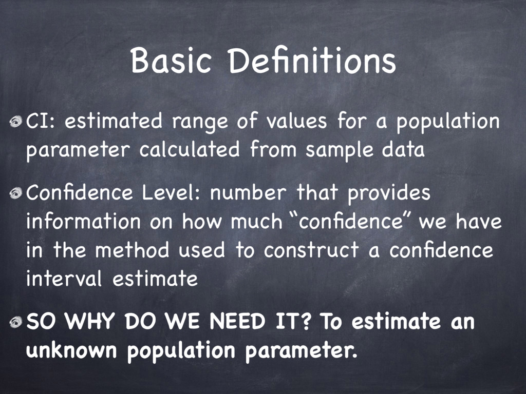
    parameter calculated from sample data Confidence Level: number that provides information on how much “confidence” we have in the method used to construct a confidence interval estimate SO WHY DO WE NEED IT? To estimate an unknown population parameter.
  3. Steps to Correctly Make a Confidence Interval 1. Assumptions 2.

    Calculations 3. Conclusions No statements!
  4. 1. Assumptions (z) Have an SRS from population (or randomly

    assigned treatments) σ known Normal (or approx. normal) distribution • Given • Large sample size (n≥30)
  5. 1. Assumptions (t) Have an SRS from population (or randomly

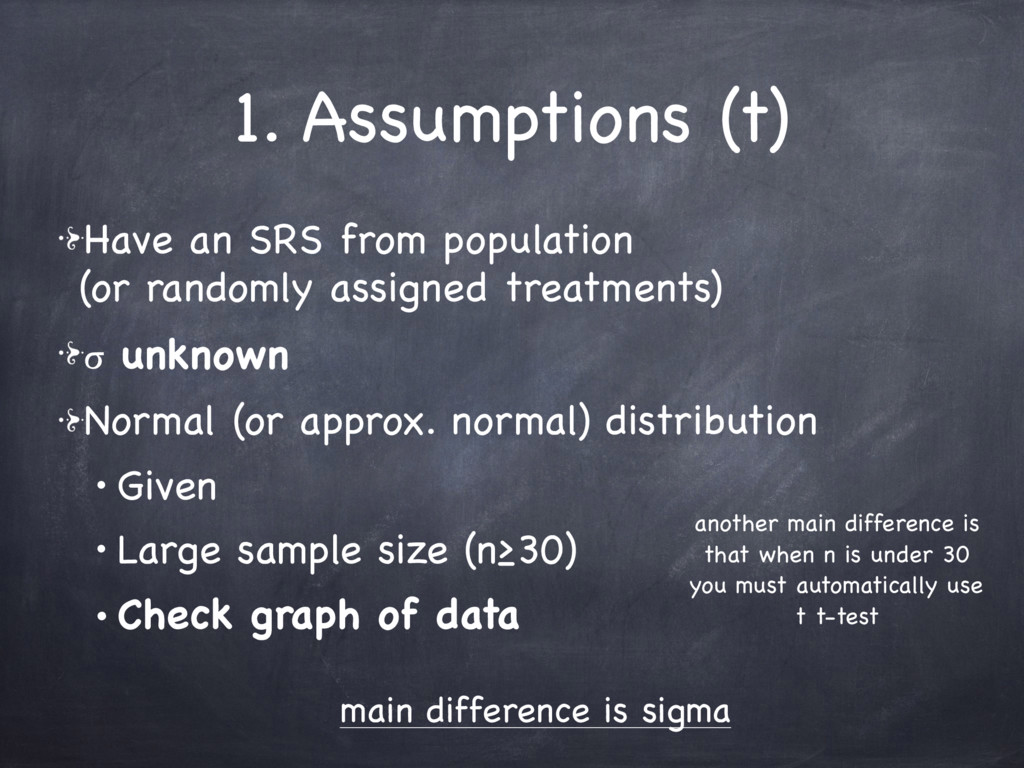
    assigned treatments) σ unknown Normal (or approx. normal) distribution • Given • Large sample size (n≥30) • Check graph of data main difference is sigma another main difference is that when n is under 30 you must automatically use t t-test
  6. 2. Calculations (z) In case of z, where the ϭ

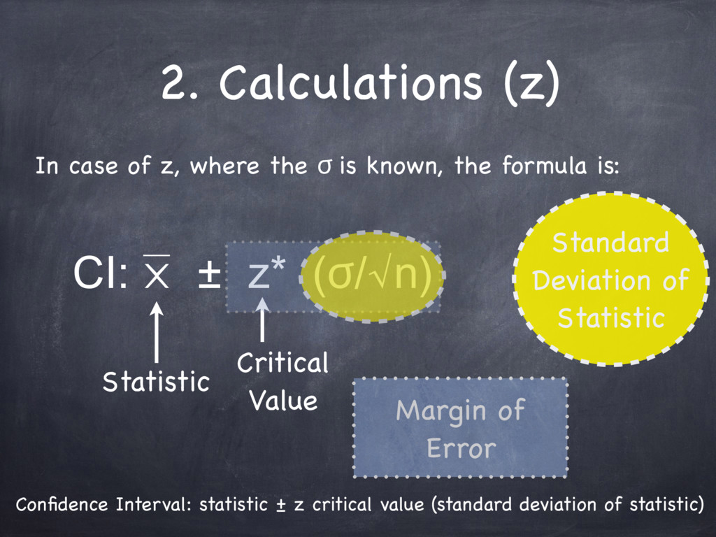
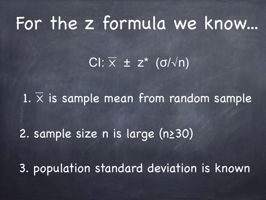
    is known, the formula is: CI: ⨉ ± z* (ϭ/√n) Statistic Critical Value Standard Deviation of Statistic Margin of Error Confidence Interval: statistic ± z critical value (standard deviation of statistic)
  7. 2. Calculations (t) In case of t, where the ϭ

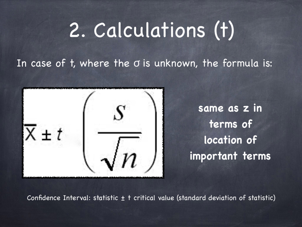
    is unknown, the formula is: Confidence Interval: statistic ± t critical value (standard deviation of statistic) same as z in terms of location of important terms
  8. 2. Calculations (t) Finding t-critical values with the table You

    use Table B: t-distributions. Look up confidence level on bottom and degress of freedom on sides where df=n-1 Example: 70% confidence when n=12 location highlighted in blue Table B t distribution critical values Tail probability p df .25 .20 .15 .10 .05 .025 .02 .01 .005 .0025 .001 .0005 1 1.000 1.376 1.963 3.078 6.314 12.71 15.89 31.82 63.66 127.3 318.3 636.6 2 .816 1.061 1.386 1.886 2.920 4.303 4.849 6.965 9.925 14.09 22.33 31.60 3 .765 .978 1.250 1.638 2.353 3.182 3.482 4.541 5.841 7.453 10.21 12.92 4 .741 .941 1.190 1.533 2.132 2.776 2.999 3.747 4.604 5.598 7.173 8.610 5 .727 .920 1.156 1.476 2.015 2.571 2.757 3.365 4.032 4.773 5.893 6.869 6 .718 .906 1.134 1.440 1.943 2.447 2.612 3.143 3.707 4.317 5.208 5.959 7 .711 .896 1.119 1.415 1.895 2.365 2.517 2.998 3.499 4.029 4.785 5.408 8 .706 .889 1.108 1.397 1.860 2.306 2.449 2.896 3.355 3.833 4.501 5.041 9 .703 .883 1.100 1.383 1.833 2.262 2.398 2.821 3.250 3.690 4.297 4.781 10 .700 .879 1.093 1.372 1.812 2.228 2.359 2.764 3.169 3.581 4.144 4.587 11 .697 .876 1.088 1.363 1.796 2.201 2.328 2.718 3.106 3.497 4.025 4.437 12 .695 .873 1.083 1.356 1.782 2.179 2.303 2.681 3.055 3.428 3.930 4.318 13 .694 .870 1.079 1.350 1.771 2.160 2.282 2.650 3.012 3.372 3.852 4.221 14 .692 .868 1.076 1.345 1.761 2.145 2.264 2.624 2.977 3.326 3.787 4.140 15 .691 .866 1.074 1.341 1.753 2.131 2.249 2.602 2.947 3.286 3.733 4.073 16 .690 .865 1.071 1.337 1.746 2.120 2.235 2.583 2.921 3.252 3.686 4.015 17 .689 .863 1.069 1.333 1.740 2.110 2.224 2.567 2.898 3.222 3.646 3.965 18 .688 .862 1.067 1.330 1.734 2.101 2.214 2.552 2.878 3.197 3.611 3.922 19 .688 .861 1.066 1.328 1.729 2.093 2.205 2.539 2.861 3.174 3.579 3.883 20 .687 .860 1.064 1.325 1.725 2.086 2.197 2.528 2.845 3.153 3.552 3.850 21 .686 .859 1.063 1.323 1.721 2.080 2.189 2.518 2.831 3.135 3.527 3.819 22 .686 .858 1.061 1.321 1.717 2.074 2.183 2.508 2.819 3.119 3.505 3.792 23 .685 .858 1.060 1.319 1.714 2.069 2.177 2.500 2.807 3.104 3.485 3.768 24 .685 .857 1.059 1.318 1.711 2.064 2.172 2.492 2.797 3.091 3.467 3.745 25 .684 .856 1.058 1.316 1.708 2.060 2.167 2.485 2.787 3.078 3.450 3.725 26 .684 .856 1.058 1.315 1.706 2.056 2.162 2.479 2.779 3.067 3.435 3.707 27 .684 .855 1.057 1.314 1.703 2.052 2.158 2.473 2.771 3.057 3.421 3.690 28 .683 .855 1.056 1.313 1.701 2.048 2.154 2.467 2.763 3.047 3.408 3.674 29 .683 .854 1.055 1.311 1.699 2.045 2.150 2.462 2.756 3.038 3.396 3.659 30 .683 .854 1.055 1.310 1.697 2.042 2.147 2.457 2.750 3.030 3.385 3.646 40 .681 .851 1.050 1.303 1.684 2.021 2.123 2.423 2.704 2.971 3.307 3.551 50 .679 .849 1.047 1.299 1.676 2.009 2.109 2.403 2.678 2.937 3.261 3.496 60 .679 .848 1.045 1.296 1.671 2.000 2.099 2.390 2.660 2.915 3.232 3.460 80 .678 .846 1.043 1.292 1.664 1.990 2.088 2.374 2.639 2.887 3.195 3.416 100 .677 .845 1.042 1.290 1.660 1.984 2.081 2.364 2.626 2.871 3.174 3.390 1000 .675 .842 1.037 1.282 1.646 1.962 2.056 2.330 2.581 2.813 3.098 3.300 ϱ .674 .841 1.036 1.282 1.645 1.960 2.054 2.326 2.576 2.807 3.091 3.291 50% 60% 70% 80% 90% 95% 96% 98% 99% 99.5% 99.8% 99.9% Confidence level C Finding t-critical values with the table CALC: 2nd > Vars > 4:invT: Then you type in invT(P,df) df=n-1 P=critical value+tail area Example: 90% confidence when n=5 CALC: invT(.90+.05, 5-1)... so invT(.95,4)= 2.1318 ≈ 2.132 Confidence Level Tail Area 80% 0.1 90% 0.05 95% 0.025 98% 0.01 99% 0.005
  9. For the z formula we know... CI: ⨉ ± z*

    (ϭ/√n) 1. ⨉ is sample mean from random sample 2. sample size n is large (n≥30) 3. population standard deviation is known
  10. For the t formula we know... CI: ⨉ ± t*

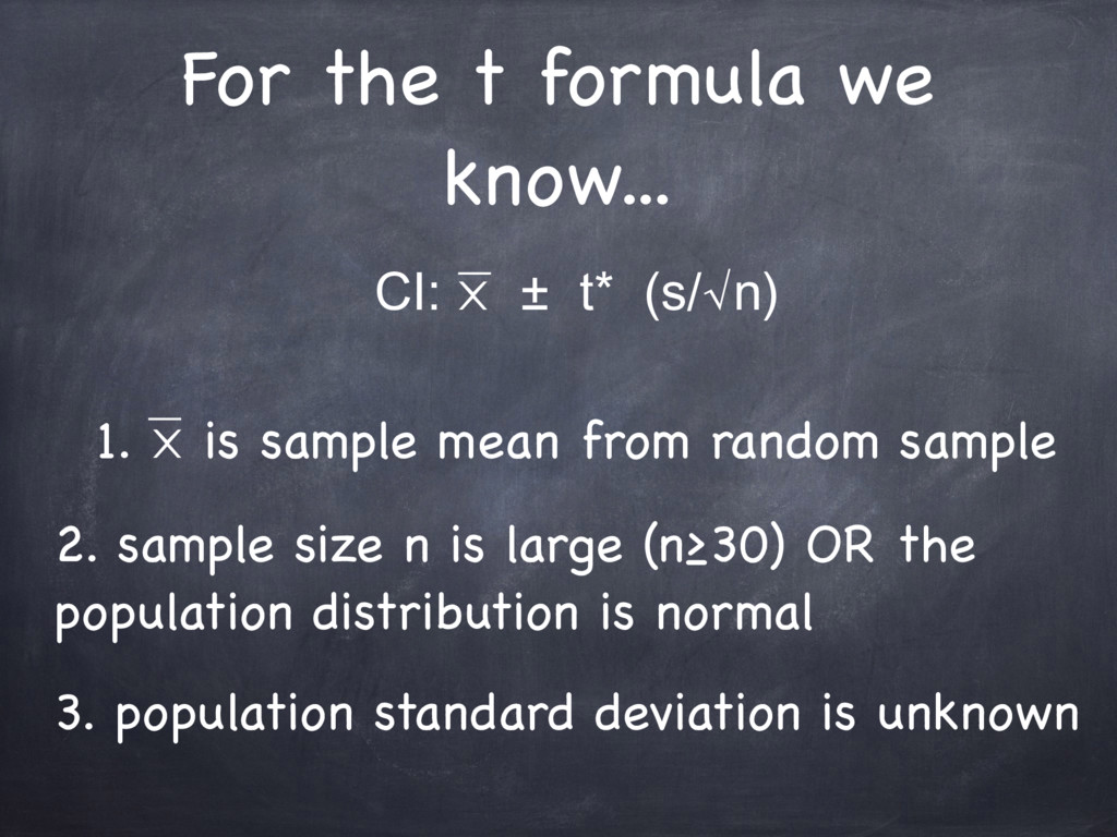
    (s/√n) 1. ⨉ is sample mean from random sample 2. sample size n is large (n≥30) OR the population distribution is normal 3. population standard deviation is unknown
  11. Confidence Levels & Corresponding z-values Confidence Level z-value 80% 1.282

    90% 1.645 95% 1.96 98% 2.326 99% 2.576 In doubt? This can all be found on the t critical values table that you receive on your AP Stat exam. 1 1.000 1.376 1.963 3.078 6.314 12.71 15.89 31.82 63.66 127.3 318.3 636.6 2 .816 1.061 1.386 1.886 2.920 4.303 4.849 6.965 9.925 14.09 22.33 31.60 3 .765 .978 1.250 1.638 2.353 3.182 3.482 4.541 5.841 7.453 10.21 12.92 4 .741 .941 1.190 1.533 2.132 2.776 2.999 3.747 4.604 5.598 7.173 8.610 5 .727 .920 1.156 1.476 2.015 2.571 2.757 3.365 4.032 4.773 5.893 6.869 6 .718 .906 1.134 1.440 1.943 2.447 2.612 3.143 3.707 4.317 5.208 5.959 7 .711 .896 1.119 1.415 1.895 2.365 2.517 2.998 3.499 4.029 4.785 5.408 8 .706 .889 1.108 1.397 1.860 2.306 2.449 2.896 3.355 3.833 4.501 5.041 9 .703 .883 1.100 1.383 1.833 2.262 2.398 2.821 3.250 3.690 4.297 4.781 10 .700 .879 1.093 1.372 1.812 2.228 2.359 2.764 3.169 3.581 4.144 4.587 11 .697 .876 1.088 1.363 1.796 2.201 2.328 2.718 3.106 3.497 4.025 4.437 12 .695 .873 1.083 1.356 1.782 2.179 2.303 2.681 3.055 3.428 3.930 4.318 13 .694 .870 1.079 1.350 1.771 2.160 2.282 2.650 3.012 3.372 3.852 4.221 14 .692 .868 1.076 1.345 1.761 2.145 2.264 2.624 2.977 3.326 3.787 4.140 15 .691 .866 1.074 1.341 1.753 2.131 2.249 2.602 2.947 3.286 3.733 4.073 16 .690 .865 1.071 1.337 1.746 2.120 2.235 2.583 2.921 3.252 3.686 4.015 17 .689 .863 1.069 1.333 1.740 2.110 2.224 2.567 2.898 3.222 3.646 3.965 18 .688 .862 1.067 1.330 1.734 2.101 2.214 2.552 2.878 3.197 3.611 3.922 19 .688 .861 1.066 1.328 1.729 2.093 2.205 2.539 2.861 3.174 3.579 3.883 20 .687 .860 1.064 1.325 1.725 2.086 2.197 2.528 2.845 3.153 3.552 3.850 21 .686 .859 1.063 1.323 1.721 2.080 2.189 2.518 2.831 3.135 3.527 3.819 22 .686 .858 1.061 1.321 1.717 2.074 2.183 2.508 2.819 3.119 3.505 3.792 23 .685 .858 1.060 1.319 1.714 2.069 2.177 2.500 2.807 3.104 3.485 3.768 24 .685 .857 1.059 1.318 1.711 2.064 2.172 2.492 2.797 3.091 3.467 3.745 25 .684 .856 1.058 1.316 1.708 2.060 2.167 2.485 2.787 3.078 3.450 3.725 26 .684 .856 1.058 1.315 1.706 2.056 2.162 2.479 2.779 3.067 3.435 3.707 27 .684 .855 1.057 1.314 1.703 2.052 2.158 2.473 2.771 3.057 3.421 3.690 28 .683 .855 1.056 1.313 1.701 2.048 2.154 2.467 2.763 3.047 3.408 3.674 29 .683 .854 1.055 1.311 1.699 2.045 2.150 2.462 2.756 3.038 3.396 3.659 30 .683 .854 1.055 1.310 1.697 2.042 2.147 2.457 2.750 3.030 3.385 3.646 40 .681 .851 1.050 1.303 1.684 2.021 2.123 2.423 2.704 2.971 3.307 3.551 50 .679 .849 1.047 1.299 1.676 2.009 2.109 2.403 2.678 2.937 3.261 3.496 60 .679 .848 1.045 1.296 1.671 2.000 2.099 2.390 2.660 2.915 3.232 3.460 80 .678 .846 1.043 1.292 1.664 1.990 2.088 2.374 2.639 2.887 3.195 3.416 100 .677 .845 1.042 1.290 1.660 1.984 2.081 2.364 2.626 2.871 3.174 3.390 1000 .675 .842 1.037 1.282 1.646 1.962 2.056 2.330 2.581 2.813 3.098 3.300 ϱ .674 .841 1.036 1.282 1.645 1.960 2.054 2.326 2.576 2.807 3.091 3.291 50% 60% 70% 80% 90% 95% 96% 98% 99% 99.5% 99.8% 99.9% Confidence level C
  12. 3. Conclusions We are __ % confident that the true

    population mean of ___ context ___ is between ___ and ___. You need to know this by memory for the AP Statistics Exam.
  13. 2. Calculations: Using the Calculator PROBLEM: We want to develop

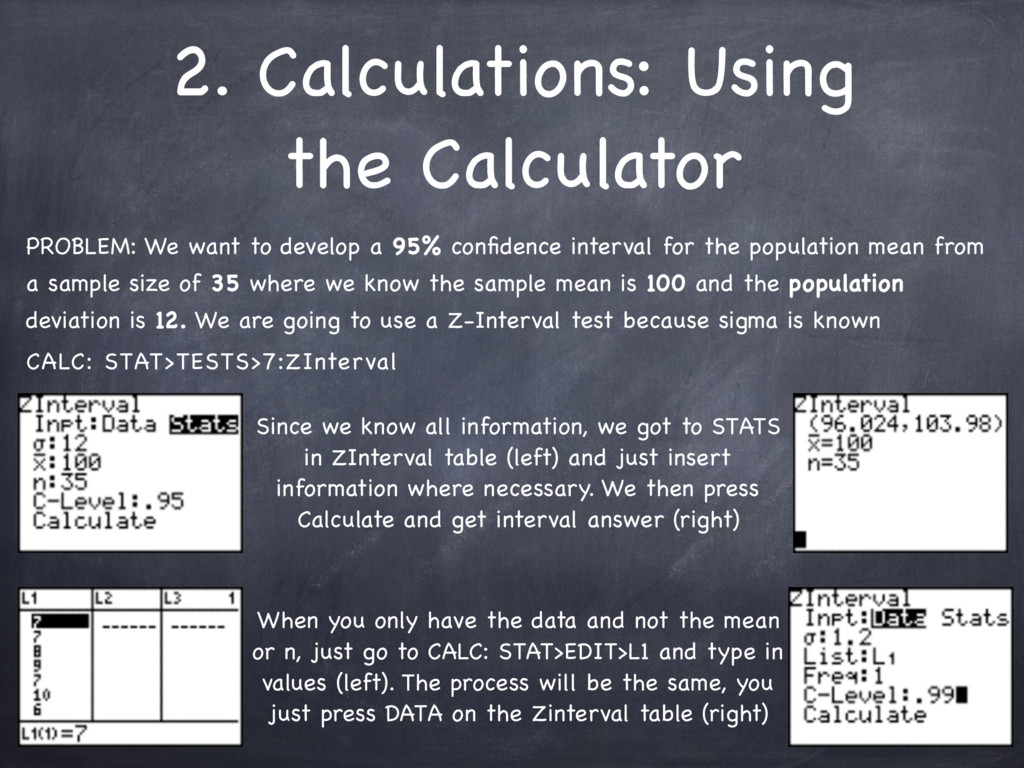
    a 95% confidence interval for the population mean from a sample size of 35 where we know the sample mean is 100 and the population deviation is 12. We are going to use a Z-Interval test because sigma is known CALC: STAT>TESTS>7:ZInterval Since we know all information, we got to STATS in ZInterval table (left) and just insert information where necessary. We then press Calculate and get interval answer (right) When you only have the data and not the mean or n, just go to CALC: STAT>EDIT>L1 and type in values (left). The process will be the same, you just press DATA on the Zinterval table (right)
  14. EXAMPLE 1: Confidence Intervals with Means: z We want to

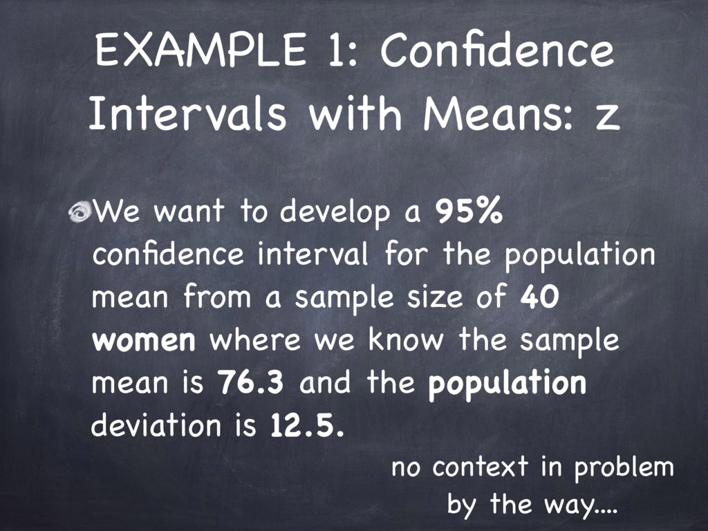
    develop a 95% confidence interval for the population mean from a sample size of 40 women where we know the sample mean is 76.3 and the population deviation is 12.5. no context in problem by the way....
  15. EXAMPLE 1: Answer CI: ⨉ ± z* (ϭ/√n) CI: 76.3

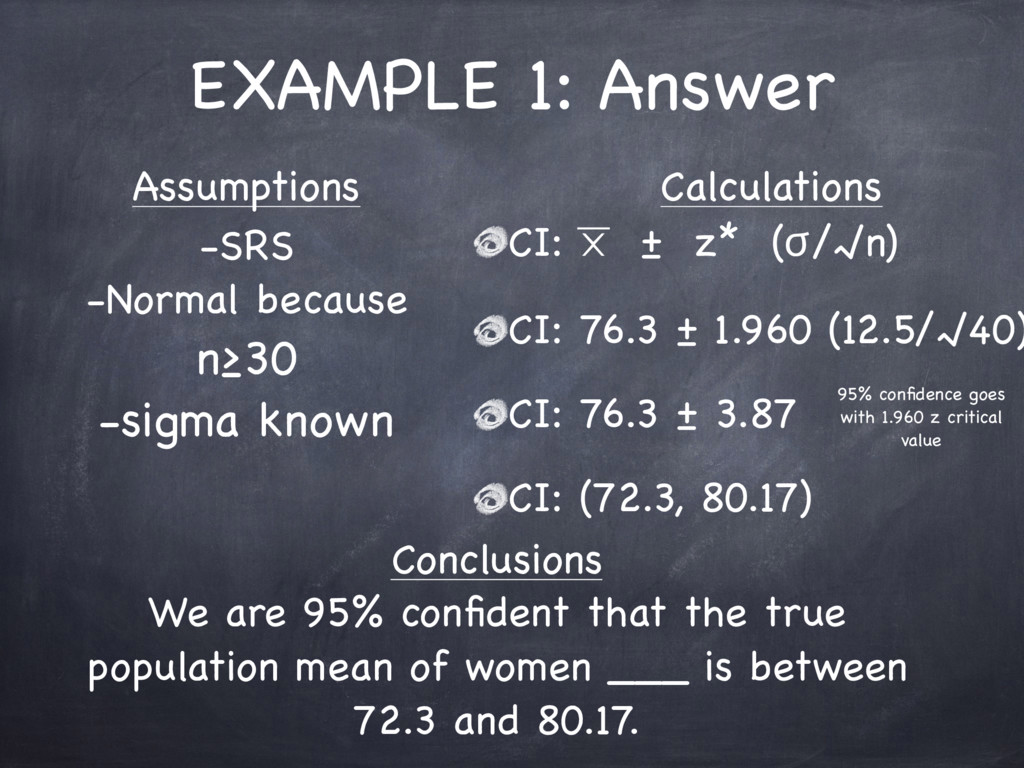
    ± 1.960 (12.5/√40) CI: 76.3 ± 3.87 CI: (72.3, 80.17) 95% confidence goes with 1.960 z critical value Calculations Assumptions -SRS -Normal because n≥30 -sigma known Conclusions We are 95% confident that the true population mean of women ___ is between 72.3 and 80.17.
  16. Determining Sample Size: 1st Option Problem: 95% confident so 1.96

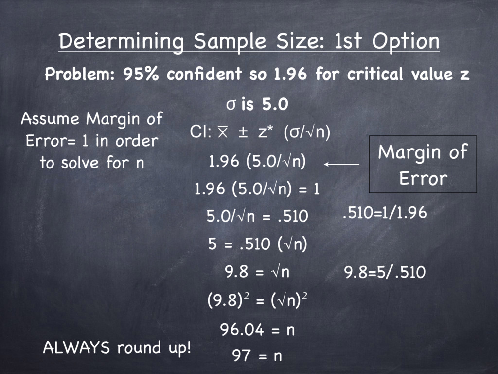
    for critical value z ϭ is 5.0 CI: ⨉ ± z* (ϭ/√n) 1.96 (5.0/√n) 1.96 (5.0/√n) = 1 5.0/√n = .510 5 = .510 (√n) 9.8 = √n (9.8)² = (√n)² 96.04 = n 97 = n Assume Margin of Error= 1 in order to solve for n Margin of Error .510=1/1.96 9.8=5/.510 ALWAYS round up!
  17. In order to solve for n you must set B,

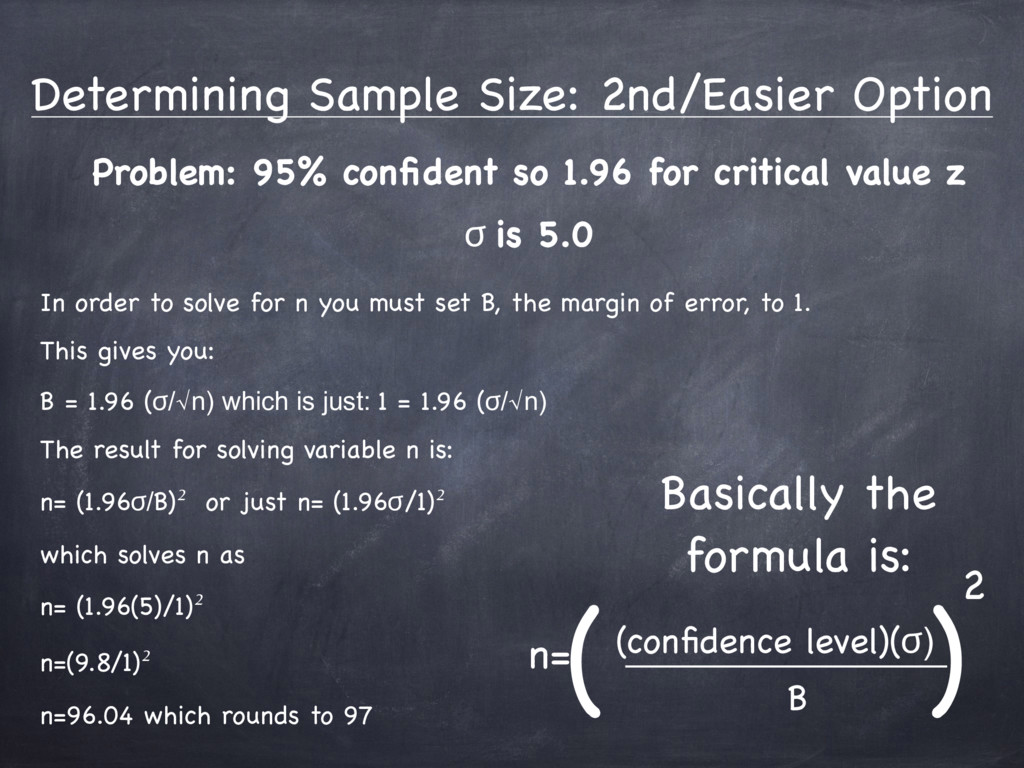
    the margin of error, to 1. This gives you: B = 1.96 (ϭ/√n) which is just: 1 = 1.96 (ϭ/√n) The result for solving variable n is: n= (1.96ϭ/B)² or just n= (1.96ϭ/1)² which solves n as n= (1.96(5)/1)² n=(9.8/1)² n=96.04 which rounds to 97 Determining Sample Size: 2nd/Easier Option Problem: 95% confident so 1.96 for critical value z ϭ is 5.0 Basically the formula is: (confidence level)(ϭ) B ( ) 2 n=
  18. Quiz Answers! 1. A: (299.89, 300.11) 2. A: At 90%

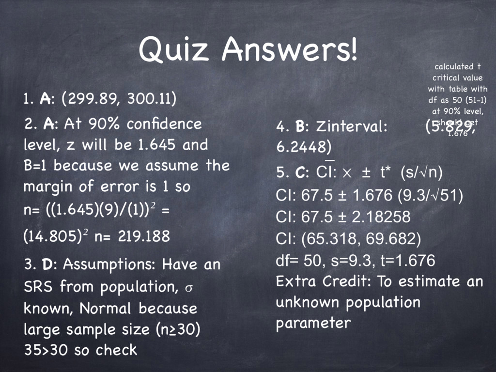
    confidence level, z will be 1.645 and B=1 because we assume the margin of error is 1 so n= ((1.645)(9)/(1))² = (14.805)² n= 219.188 3. D: Assumptions: Have an SRS from population, σ known, Normal because large sample size (n≥30) 35>30 so check 4. B: Zinterval: (5.829, 6.2448) 5. C: CI: ⨉ ± t* (s/√n) CI: 67.5 ± 1.676 (9.3/√51) CI: 67.5 ± 2.18258 CI: (65.318, 69.682) df= 50, s=9.3, t=1.676 Extra Credit: To estimate an unknown population parameter calculated t critical value with table with df as 50 (51-1) at 90% level, should get 1.676
  19. Sources " Z - C o n f i d

    e n ce I nte r va l. " P re n h a l l. N.p. , n . d . We b. 2 3 M a y 2 0 1 1 . < htt p : //w w w.pre n h a l l.co m /e s m /a p p / ca lc _ v 2/ca lc u lato r/m e d ia li b /Te c h n o lo g y/ D o c u m e nt s / T I- 8 3/d e s c _ p a g e s /z _ co n f _ i nte r. ht m l > M a s s ey, Tiffa n y. "C o n f i d e n ce I nte r va l N ote s. " A P S tat i st ic s: B e l l 7. M H S M at h D e p a r t m e nt. M a u r y H i g h S c h o o l, N o r fo l k , VA. 2 0 1 0 -2 0 1 1 . L e ct u re s. Slide 13 Rest of Slides