Upgrade to Pro — share decks privately, control downloads, hide ads and more …

Measuring starspot physical properties with Kepler/K2 and high resolution near IR spectroscopy

gully
October 25, 2018
130

Measuring starspot physical properties with Kepler/K2 and high resolution near IR spectroscopy

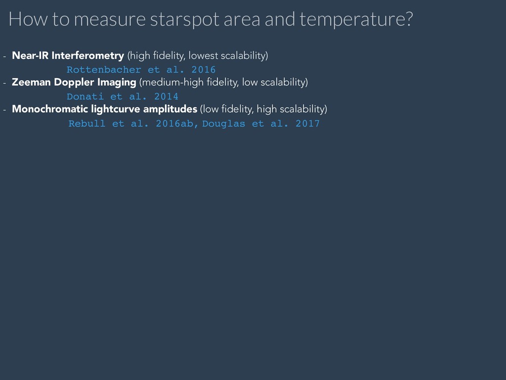
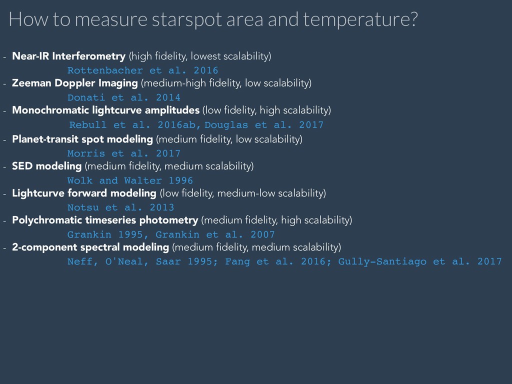
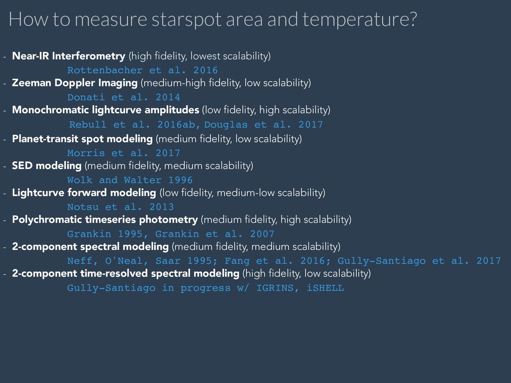
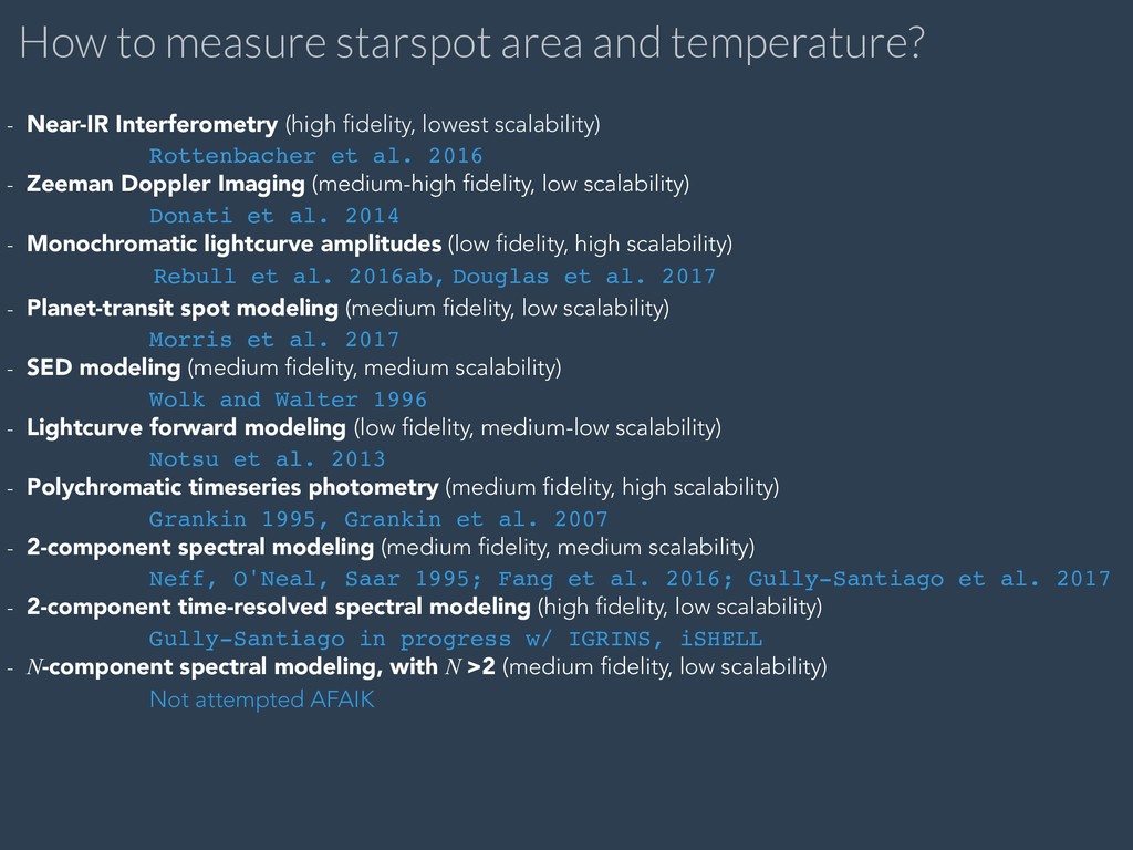
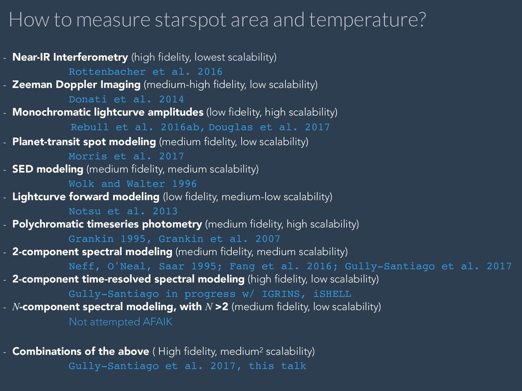
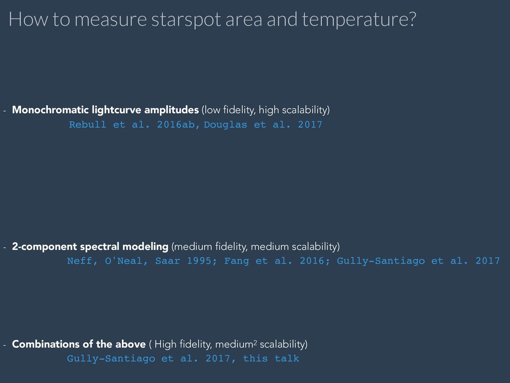
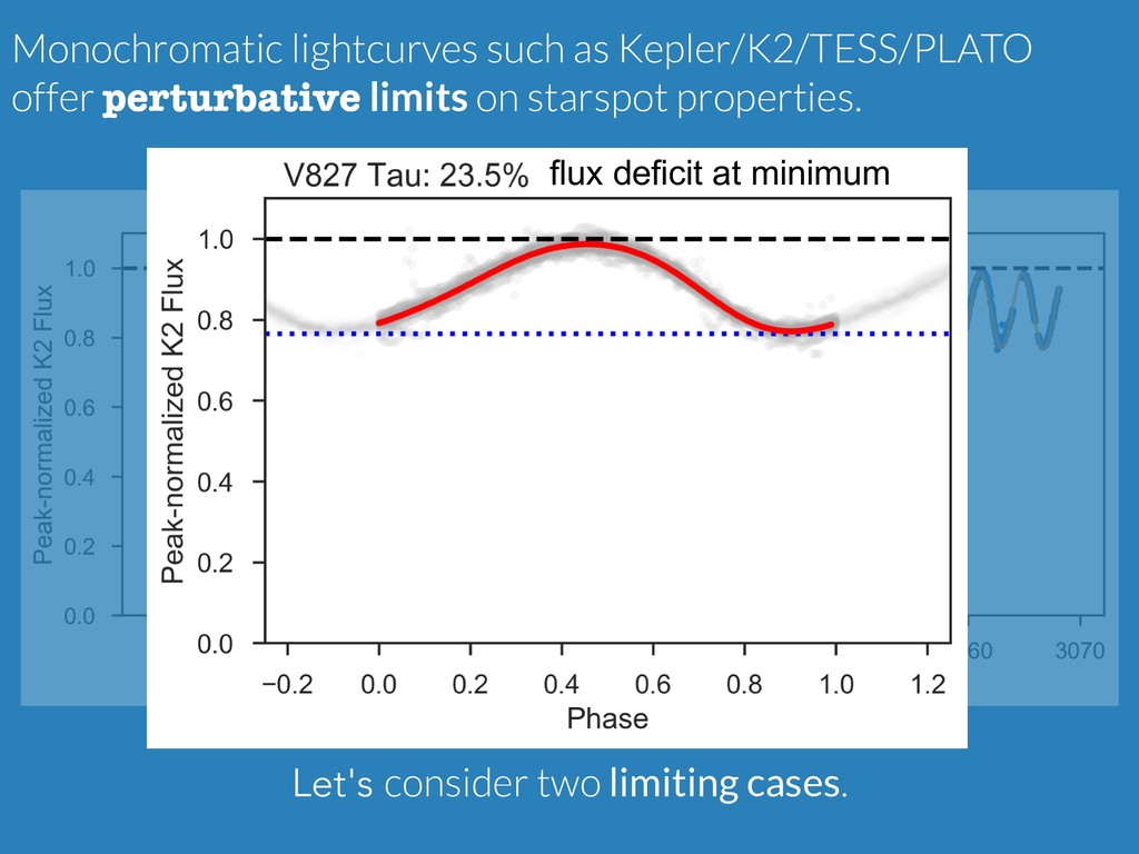
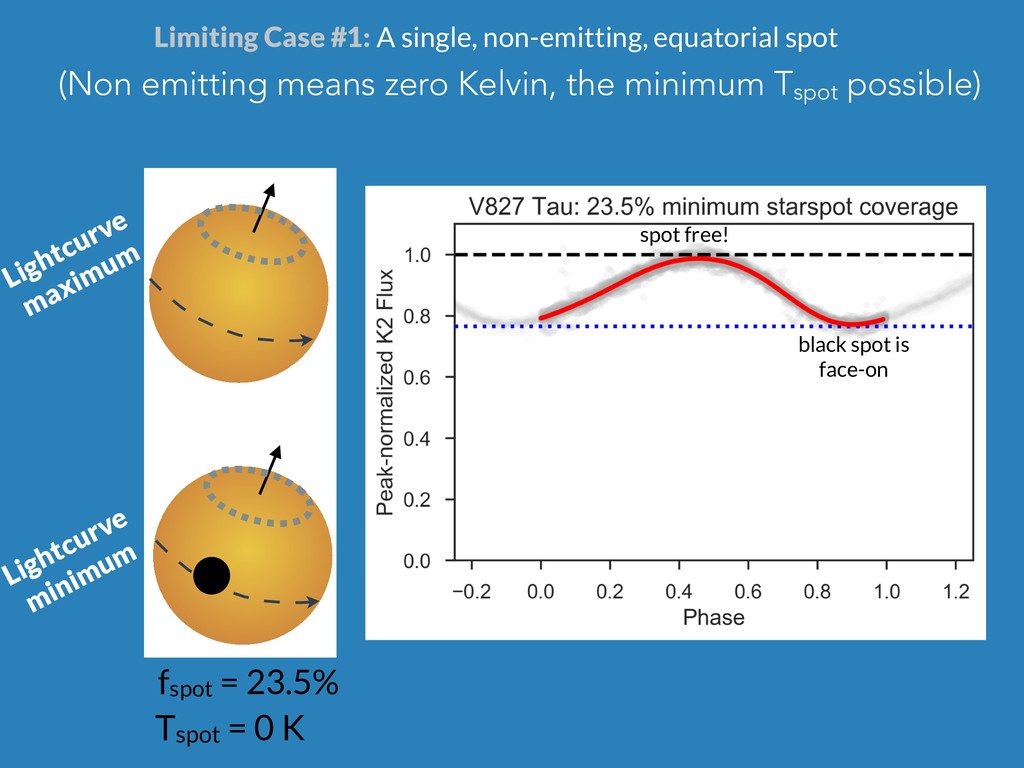
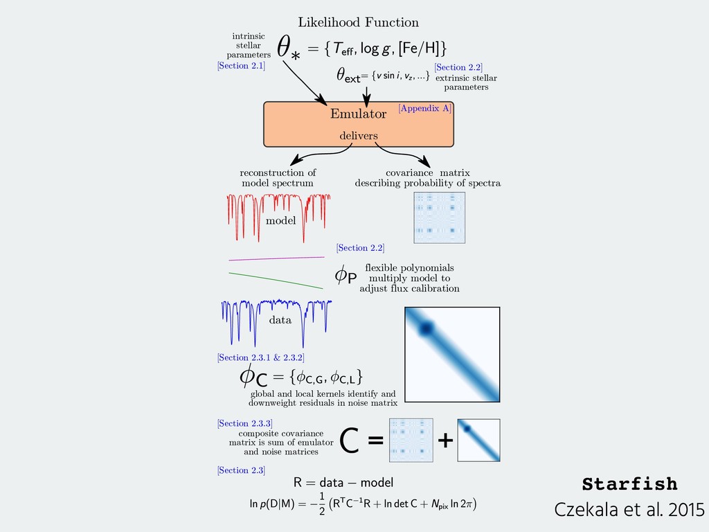
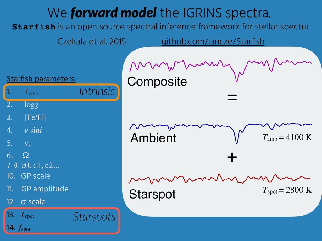
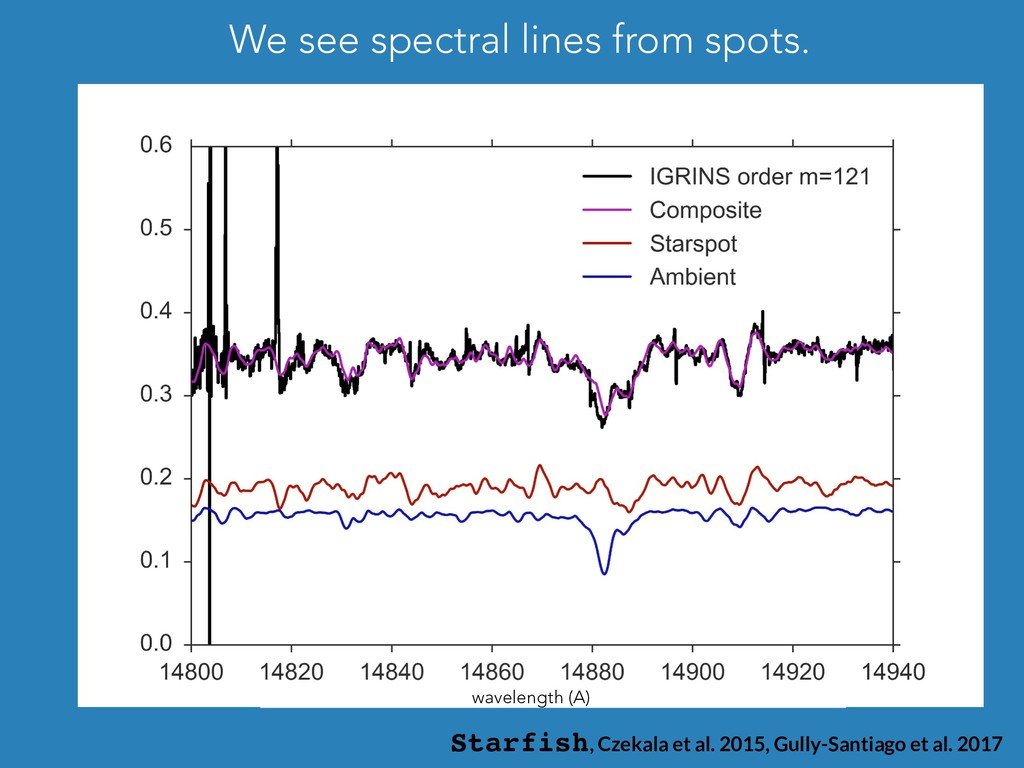
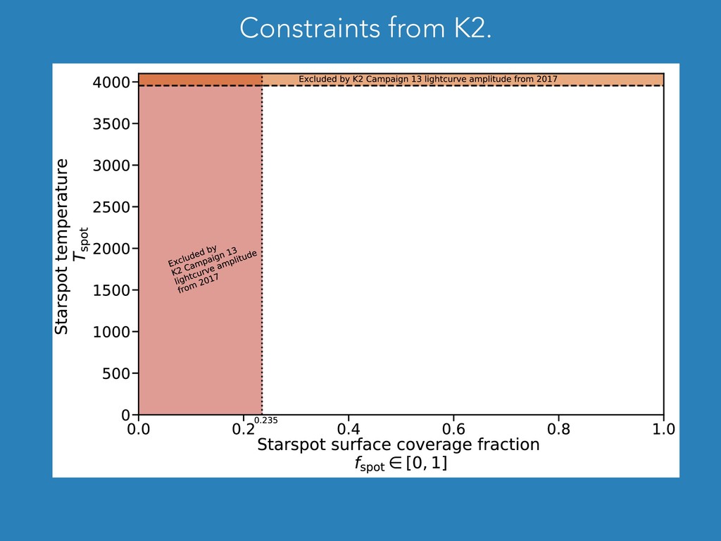
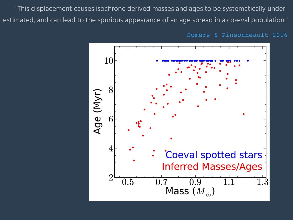
Active longitudes at high latitudes on inclined stars remain largely unquantified owing to their zero or near-zero temporal variability. The areal coverage fraction of starspots possessing non-standard geometries (i.e. dissimilar from sunspots) may be significantly underestimated. In this talk, I contrast the scalability and fidelity of complementary observational techniques for quantifying starspot areal coverage fractions and temperatures. I demonstrate the limited-albeit-informative constraining power of precision monochromatic lightcurves. I have developed a flexible two-component spectral inference framework to measure starspot area and temperature from composite spectra of spotted stars. The framework provides exceptional constraints on the total starspot coverage of a stellar hemisphere, especially when combined with high-resolution high-bandwidth near infrared spectroscopy, such as IGRINS or iSHELL. I propose a path forward for evaluating starspot-induced biases in star cluster ages, eclipsing binary radii, and exoplanet transit depths.

gully

October 25, 2018
Tweet

Transcript

  1. Measuring starspot physical properties with Kepler/K2 and high resolution near

    IR spectroscopy Michael Gully-Santiago Kepler/K2 Guest Observer Office NASA Ames Research Center PLATO-ESP 2018 workshop Stellar Variability and the Characterization of Small Planets October 24, 2018
  2. **For sun-like stars in Kepler prime, Rapid rotators spot tend

    to be dominated. Slow rotators faculae Montet, Tovar, Foreman-Mackey 2017 The techniques described in this talk apply equally to spots or faculae, but I will focus on spots. { }
  3. What can you measure? = To zeroth order, spots are

    simply a localized absence of flux. To first order, spots are localized photospheres indexed by cooler "effective temperatures". To second order, there are correction terms for depth, Zeeman, and viewing angle effects. •Starspot area •Starspot temperature
  4. What can you measure? = + To zeroth order, spots

    are simply a localized absence of flux. To first order, spots are localized photospheres indexed by cooler "effective temperatures". To second order, there are correction terms for depth, Zeeman, and viewing angle effects. •Starspot area •Starspot temperature
  5. What can you measure? = + To zeroth order, spots

    are simply a localized absence of flux. To first order, spots are localized photospheres indexed by cooler "effective temperatures". To second order, there are correction terms for depth, Zeeman, and viewing angle effects. •Starspot area •Starspot temperature + ...
  6. What can you measure? = + To zeroth order, spots

    are simply a localized absence of flux. To first order, spots are localized photospheres indexed by cooler "effective temperatures". To second order, there are correction terms for depth, Zeeman, and viewing angle effects. •Starspot area •Starspot temperature
  7. All spotted stars must (approximately) populate this plot. Definitions Areas:

    fspot = Aspot/Astar Temperatures: Tspot < Tambient (Teff gets redefined!)
  8. Key distinction among starspot measurement techniques Perturbative- Capture "merely" perturbations

    arising from rotational modulation from longitudinal asymmetries in starspot location detects starspot A A B Full stellar disk- Captures all the starspot flux at a given hemisphere epoch, regardless of longitudinal/latitudinal distribution, distinguishing starspots through some other means, e.g. spatially or spectrally detects starspots A & B
  9. How to measure starspot area and temperature? - Near-IR Interferometry

    (high fidelity, lowest scalability) Rottenbacher et al. 2016 - Zeeman Doppler Imaging (medium-high fidelity, low scalability) Donati et al. 2014 - Monochromatic lightcurve amplitudes (low fidelity, high scalability) Rebull et al. 2016ab, Douglas et al. 2017 - Planet-transit spot modeling (medium fidelity, low scalability) Morris et al. 2017 - SED modeling (medium fidelity, medium scalability) Wolk and Walter 1996 - Lightcurve forward modeling (low fidelity, medium-low scalability) Notsu et al. 2013 - Polychromatic timeseries photometry (medium fidelity, high scalability) Grankin 1995, Grankin et al. 2007 - 2-component spectral modeling (medium fidelity, medium scalability) Neff, O'Neal, Saar 1995; Fang et al. 2016; Gully-Santiago et al. 2017 - 2-component time-resolved spectral modeling (high fidelity, low scalability) Gully-Santiago in progress w/ IGRINS, iSHELL - N-component spectral modeling, with N >2 (medium fidelity, low scalability) Not attempted AFAIK - Combinations of the above ( High fidelity, medium2 scalability) Gully-Santiago et al. 2017, this talk
  10. How to measure starspot area and temperature? - Near-IR Interferometry

    (high fidelity, lowest scalability) Rottenbacher et al. 2016 - Zeeman Doppler Imaging (medium-high fidelity, low scalability) Donati et al. 2014 - Monochromatic lightcurve amplitudes (low fidelity, high scalability) Rebull et al. 2016ab, Douglas et al. 2017 - Planet-transit spot modeling (medium fidelity, low scalability) Morris et al. 2017 - SED modeling (medium fidelity, medium scalability) Wolk and Walter 1996 - Lightcurve forward modeling (low fidelity, medium-low scalability) Notsu et al. 2013 - Polychromatic timeseries photometry (medium fidelity, high scalability) Grankin 1995, Grankin et al. 2007 - 2-component spectral modeling (medium fidelity, medium scalability) Neff, O'Neal, Saar 1995; Fang et al. 2016; Gully-Santiago et al. 2017 - 2-component time-resolved spectral modeling (high fidelity, low scalability) Gully-Santiago in progress w/ IGRINS, iSHELL - N-component spectral modeling, with N >2 (medium fidelity, low scalability) Not attempted AFAIK - Combinations of the above ( High fidelity, medium2 scalability) Gully-Santiago et al. 2017, this talk
  11. How to measure starspot area and temperature? - Near-IR Interferometry

    (high fidelity, lowest scalability) Rottenbacher et al. 2016 - Zeeman Doppler Imaging (medium-high fidelity, low scalability) Donati et al. 2014 - Monochromatic lightcurve amplitudes (low fidelity, high scalability) Rebull et al. 2016ab, Douglas et al. 2017 - Planet-transit spot modeling (medium fidelity, low scalability) Morris et al. 2017 - SED modeling (medium fidelity, medium scalability) Wolk and Walter 1996 - Lightcurve forward modeling (low fidelity, medium-low scalability) Notsu et al. 2013 - Polychromatic timeseries photometry (medium fidelity, high scalability) Grankin 1995, Grankin et al. 2007 - 2-component spectral modeling (medium fidelity, medium scalability) Neff, O'Neal, Saar 1995; Fang et al. 2016; Gully-Santiago et al. 2017 - 2-component time-resolved spectral modeling (high fidelity, low scalability) Gully-Santiago in progress w/ IGRINS, iSHELL - N-component spectral modeling, with N >2 (medium fidelity, low scalability) Not attempted AFAIK - Combinations of the above ( High fidelity, medium2 scalability) Gully-Santiago et al. 2017, this talk
  12. How to measure starspot area and temperature? - Near-IR Interferometry

    (high fidelity, lowest scalability) Rottenbacher et al. 2016 - Zeeman Doppler Imaging (medium-high fidelity, low scalability) Donati et al. 2014 - Monochromatic lightcurve amplitudes (low fidelity, high scalability) Rebull et al. 2016ab, Douglas et al. 2017 - Planet-transit spot modeling (medium fidelity, low scalability) Morris et al. 2017 - SED modeling (medium fidelity, medium scalability) Wolk and Walter 1996 - Lightcurve forward modeling (low fidelity, medium-low scalability) Notsu et al. 2013 - Polychromatic timeseries photometry (medium fidelity, high scalability) Grankin 1995, Grankin et al. 2007 - 2-component spectral modeling (medium fidelity, medium scalability) Neff, O'Neal, Saar 1995; Fang et al. 2016; Gully-Santiago et al. 2017 - 2-component time-resolved spectral modeling (high fidelity, low scalability) Gully-Santiago in progress w/ IGRINS, iSHELL - N-component spectral modeling, with N >2 (medium fidelity, low scalability) Not attempted AFAIK - Combinations of the above ( High fidelity, medium2 scalability) Gully-Santiago et al. 2017, this talk
  13. How to measure starspot area and temperature? - Near-IR Interferometry

    (high fidelity, lowest scalability) Rottenbacher et al. 2016 - Zeeman Doppler Imaging (medium-high fidelity, low scalability) Donati et al. 2014 - Monochromatic lightcurve amplitudes (low fidelity, high scalability) Rebull et al. 2016ab, Douglas et al. 2017 - Planet-transit spot modeling (medium fidelity, low scalability) Morris et al. 2017 - SED modeling (medium fidelity, medium scalability) Wolk and Walter 1996 - Lightcurve forward modeling (low fidelity, medium-low scalability) Notsu et al. 2013 - Polychromatic timeseries photometry (medium fidelity, high scalability) Grankin 1995, Grankin et al. 2007 - 2-component spectral modeling (medium fidelity, medium scalability) Neff, O'Neal, Saar 1995; Fang et al. 2016; Gully-Santiago et al. 2017 - 2-component time-resolved spectral modeling (high fidelity, low scalability) Gully-Santiago in progress w/ IGRINS, iSHELL - N-component spectral modeling, with N >2 (medium fidelity, low scalability) Not attempted AFAIK - Combinations of the above ( High fidelity, medium2 scalability) Gully-Santiago et al. 2017, this talk
  14. How to measure starspot area and temperature? - Near-IR Interferometry

    (high fidelity, lowest scalability) Rottenbacher et al. 2016 - Zeeman Doppler Imaging (medium-high fidelity, low scalability) Donati et al. 2014 - Monochromatic lightcurve amplitudes (low fidelity, high scalability) Rebull et al. 2016ab, Douglas et al. 2017 - Planet-transit spot modeling (medium fidelity, low scalability) Morris et al. 2017 - SED modeling (medium fidelity, medium scalability) Wolk and Walter 1996 - Lightcurve forward modeling (low fidelity, medium-low scalability) Notsu et al. 2013 - Polychromatic timeseries photometry (medium fidelity, high scalability) Grankin 1995, Grankin et al. 2007 - 2-component spectral modeling (medium fidelity, medium scalability) Neff, O'Neal, Saar 1995; Fang et al. 2016; Gully-Santiago et al. 2017 - 2-component time-resolved spectral modeling (high fidelity, low scalability) Gully-Santiago in progress w/ IGRINS, iSHELL - N-component spectral modeling, with N >2 (medium fidelity, low scalability) Not attempted AFAIK - Combinations of the above ( High fidelity, medium2 scalability) Gully-Santiago et al. 2017, this talk
  15. How to measure starspot area and temperature? - Near-IR Interferometry

    (high fidelity, lowest scalability) Rottenbacher et al. 2016 - Zeeman Doppler Imaging (medium-high fidelity, low scalability) Donati et al. 2014 - Monochromatic lightcurve amplitudes (low fidelity, high scalability) Rebull et al. 2016ab, Douglas et al. 2017 - Planet-transit spot modeling (medium fidelity, low scalability) Morris et al. 2017 - SED modeling (medium fidelity, medium scalability) Wolk and Walter 1996 - Lightcurve forward modeling (low fidelity, medium-low scalability) Notsu et al. 2013 - Polychromatic timeseries photometry (medium fidelity, high scalability) Grankin 1995, Grankin et al. 2007 - 2-component spectral modeling (medium fidelity, medium scalability) Neff, O'Neal, Saar 1995; Fang et al. 2016; Gully-Santiago et al. 2017 - 2-component time-resolved spectral modeling (high fidelity, low scalability) Gully-Santiago in progress w/ IGRINS, iSHELL - N-component spectral modeling, with N >2 (medium fidelity, low scalability) Not attempted AFAIK - Combinations of the above ( High fidelity, medium2 scalability) Gully-Santiago et al. 2017, this talk
  16. How to measure starspot area and temperature? - Near-IR Interferometry

    (high fidelity, low scalability) Rottenbacher et al. 2016 - Zeeman Doppler Imaging (medium-high fidelity, low scalability) Donati et al. 2014 - Monochromatic lightcurve amplitudes (low fidelity, high scalability) Rebull et al. 2016ab, Douglas et al. 2017 - Planet-transit spot modeling (medium fidelity, low scalability) Morris et al. 2017 - SED modeling (medium-low fidelity, medium scalability) Wolk and Walter 1996 - Lightcurve forward modeling (low fidelity, medium-low scalability) Notsu et al. 2013 - Polychromatic timeseries photometry (medium fidelity, high scalability) Grankin 1995, Grankin et al. 2007 - 2-component spectral modeling (medium fidelity, medium scalability) Neff, O'Neal, Saar 1995; Fang et al. 2016; Gully-Santiago et al. 2017 - 2-component time-resolved spectral modeling (high fidelity, low scalability) Gully-Santiago in progress w/ IGRINS, iSHELL - N-component spectral modeling, with N >2 (medium fidelity, low scalability) Not attempted AFAIK - Combinations of the above ( High fidelity, medium2 scalability) Gully-Santiago et al. 2017, this talk
  17. Monochromatic lightcurves such as Kepler/K2/TESS/PLATO offer perturbative limits on starspot

    properties. flux deficit at minimum Let's consider two limiting cases.
  18. Single, zero Kelvin, non-emitting starspot ghtcurve aximum ghtcurve inimum Pathologically

    Asymmetric Two- Temperature Hemispheres Equator-on Polar Starspot that cyclicly grows and shrinks Lightcurve maximum Lightcurve minimum fspot = 23.5% Tspot = 0 K Limiting Case #1: A single, non-emitting, equatorial spot spot free! black spot is face-on (Non emitting means zero Kelvin, the minimum Tspot possible)
  19. ghtcurve ghtcurve Lightcurve maximum Lightcurve minimum fspot = 23.5% Tspot

    = 0 K Limiting Case #1: A single, non-emitting, equatorial spot spot free! black spot is face-on (Non emitting means zero Kelvin, the minimum Tspot possible)
  20. ghtcurve ghtcurve Lightcurve maximum Lightcurve minimum fspot = 23.5% Tspot

    = 0 K Limiting Case #1: A single, non-emitting, equatorial spot spot free! black spot is face-on (Non emitting means zero Kelvin, the minimum Tspot possible) Coverage fractions smaller than 23.5% would not block enough flux.
  21. rspot Pathologically Asymmetric Two- Temperature Hemispheres Equator-on Polar Starspot that

    cyclicly grows and shrinks High latitude, geometrically foreshortened circumpolar active longitude starspot Lightcurve maximum Lightcurve minimum fspot = 100% Tspot = 3955 K Limiting Case #2: A hemisphere covered entirely with spots with Tspot spot free! cool hemisphere is face on (One hemisphere has fspot =%, maximum fspot possible.) 3955 K minimum Tspot In the Kepler bandpass, a ~3955 K hemisphere produces a 23.5% loss of flux compared to the 4100 K hemisphere.
  22. Lightcurve maximum Lightcurve minimum fspot = 100% Tspot = 3955

    K Limiting Case #2: A hemisphere covered entirely with spots with Tspot spot free! cool hemisphere is face on (One hemisphere has fspot =%, maximum fspot possible.) 3955 K minimum Tspot
  23. Lightcurve maximum Lightcurve minimum fspot = 100% Tspot = 3955

    K Limiting Case #2: A hemisphere covered entirely with spots with Tspot spot free! cool hemisphere is face on (One hemisphere has fspot =%, maximum fspot possible.) 3955 K minimum Tspot Spots warmer than 3955 K would not produce a large enough flux decrement.
  24. High resolution, high bandwidth, near-IR spectroscopy collects spot emission over

    the full stellar disk. IGRINS is an R=45,000 spectrograph covering all of H and K in a single exposure. It uses silicon immersion gratings that I developed and tested.
  25. How does one spectrally decompose an observed spectrum into starspots

    and ambient components, honoring the observation noise and uncertainties in stellar, spot, and calibration parameters?
  26. Likelihood Function intrinsic stellar parameters flexible polynomials multiply model to

    adjust flux calibration data global and local kernels identify and downweight residuals in noise matrix + = Emulator reconstruction of model spectrum covariance matrix describing probability of spectra composite covariance matrix is sum of emulator and noise matrices model [Appendix A] extrinsic stellar parameters delivers [Section 2.2] [Section 2.3] [Section 2.3.1 & 2.3.2] [Section 2.3.3] [Section 2.2] [Section 2.1] Starfish Czekala et al. 2015
  27. We forward model the IGRINS spectra. Starfish is an open

    source spectral inference framework for stellar spectra. Czekala et al. 2015 github.com/iancze/Starfish Starfish parameters: 1. Tamb 2. logg 3. [Fe/H] 4. v sini 5. vz 6. Ω 7-9. c0, c1, c2... 10. GP scale 11. GP amplitude 12. σ scale 13. Tspot 14. fspot Intrinsic Starspots = + Composite Ambient Starspot Tspot = 2800 K Tamb = 4100 K
  28. Constraints from K2 and IGRINS Each point is an independent

    estimate from different IGRINS spectral orders.
  29. Reaching to smaller spot coverage fractions We have currently developing

    this technique on young stars and evolved stars with large spot coverage fractions. What about planet hosts with solar-like (small) spots? In this case, the model imperfections matter more; these demerits are partially compensated with more data -- existing PRV data should be adequate.
  30. https://github.com/iancze/PSOAP Path forward: data-driven spot spectra models Analogous to spectroscopic

    binary applications. Offers some advantages over cross-correlation techniques. Capable of mapping much smaller filling factors Czekala et al. 2017
  31. Conclusions - We saw a framework to measure starspot area

    and temperature. - The method combines precision lightcurves and near-IR spectroscopy. - We applied the method to large-amplitude young stars, finding large spots. - We overviewed alternative methods that yield differing levels of fidelity and scalability. - We distinguished between perturbative methods and those sensitive to all spot emission. Conceivable topics for discussion - What about faculae? - To what extent can the methods developed here be applied to sun-like stars? - What is the path forward for mitigating the Transit Light Source Effect? - Are we biasing our thinking of starspots to solar-like geometries? What about polar spots? What about inclination effects? - At what turnover point(s) does suppression of convective blueshift become the dominant source of RV jitter?
  32. Impacts for PLATO design - Stellar "noise" and planet signals

    usually occur at much different timescales. - Effects that are negligible for planet transit timescales may still harm stellar signals - Sub-pixel flat field - Secular PSF variations on timescales of days - months, chromatic dependence - Differential velocity aberration arXiv:1806.07430 Direct measurement of the intra-pixel response function of the Kepler Space Telescope's CCDs Vorobiev et al. 2018 Design your data collection to anticipate self calibration
  33. Conclusions - We saw a framework to measure starspot area

    and temperature. - The method combines precision lightcurves and near-IR spectroscopy. - We applied the method to large-amplitude young stars, finding large spots. - We overviewed alternative methods that yield differing levels of fidelity and scalability. - We distinguished between perturbative methods and those sensitive to all spot emission. Conceivable topics for discussion - What about faculae? - To what extent can the methods developed here be applied to sun-like stars? - What is the path forward for mitigating the Transit Light Source Effect? - Are we biasing our thinking of starspots to solar-like geometries? What about polar spots? What about inclination effects? - At what turnover point(s) does suppression of convective blueshift become the dominant source of RV jitter?
  34. Pre-transit Stellar Disk is the Assumed Light Source Actual Light

    Source is the Chord Defined by the Planet’s Projection The Transit Light Source Effect Spectral Difference due to Different Spot/Faculae Contributions Contaminates Transit Spectrum Observed Transit Spectrum True Planetary Spectrum Rackham, Apai, Giampapa 2018
  35. "...mass, composition, and age do not uniquely specify the Hertzsprung-

    Russell diagram location of pre-MS stars." Somers & Pinsonneault 2015
  36. "This displacement causes isochrone derived masses and ages to be

    systematically under- estimated, and can lead to the spurious appearance of an age spread in a co-eval population." Somers & Pinsonneault 2016
  37. The disk lifetime limits the planet formation timescale. Haisch et

    al. 2001, Alexander & Armitage 2009, Kraus et al. 2012 How accurate are cluster ages?