Kepler/K2 driftscan FFI analysis

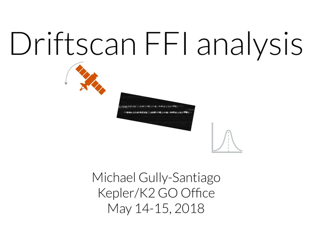
We recently carried out a short pilot program on a new, experimental data collection mode for the Kepler Space Telescope. We collected Full Frame Images (FFIs) while the field of view was drifting at ~0.3-0.5 arcseconds per second, much higher than during normal science operations. We are calling the resulting images driftscan Full Frame Images. These images may facilitate in-situ focal plane characterization and self-calibration, ultimately useful for scene modeling and Point Spread Function (PSF) photometry in crowded regions like star clusters or in extended objects.

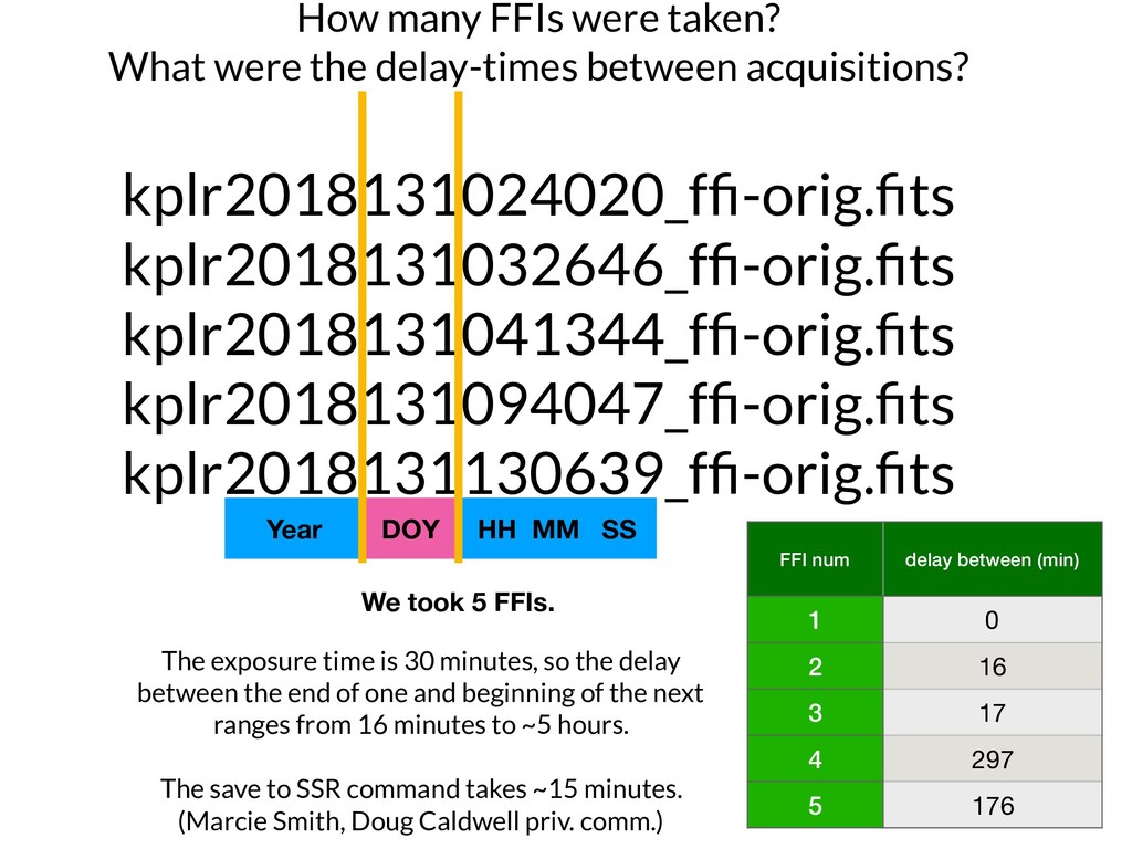
Five driftscan FFIs we acquired on May 10-11, 2018, during the K2 Campaign 17 (C17) Deep Space Network (DSN) downlink, after all C17 science data had been safely telemetered and spare DSN time remained. In this configuration, the spacecraft antenna points towards Earth; driftscan FFIs are telemetered back immediately after acquisition.

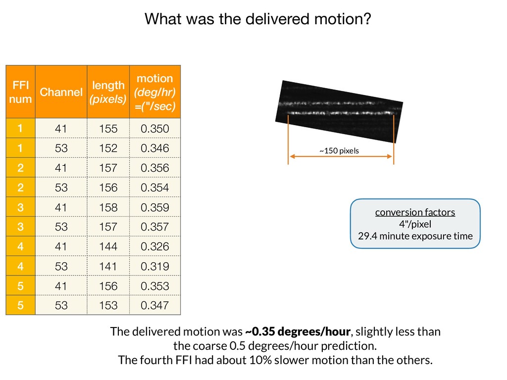
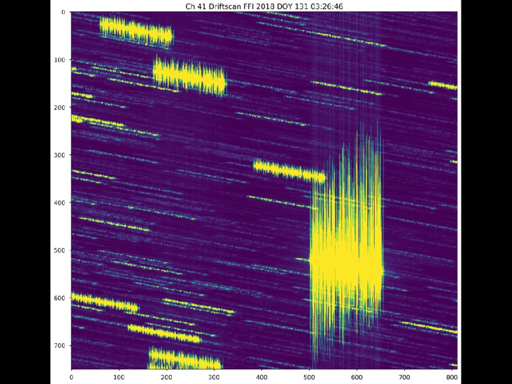
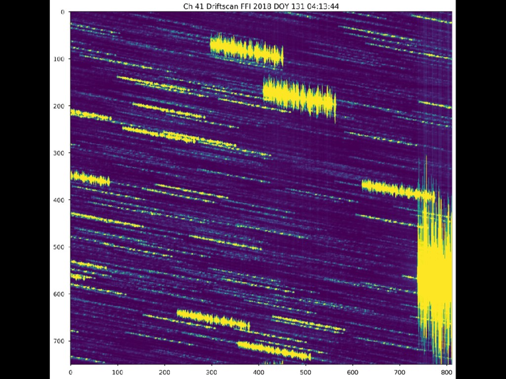
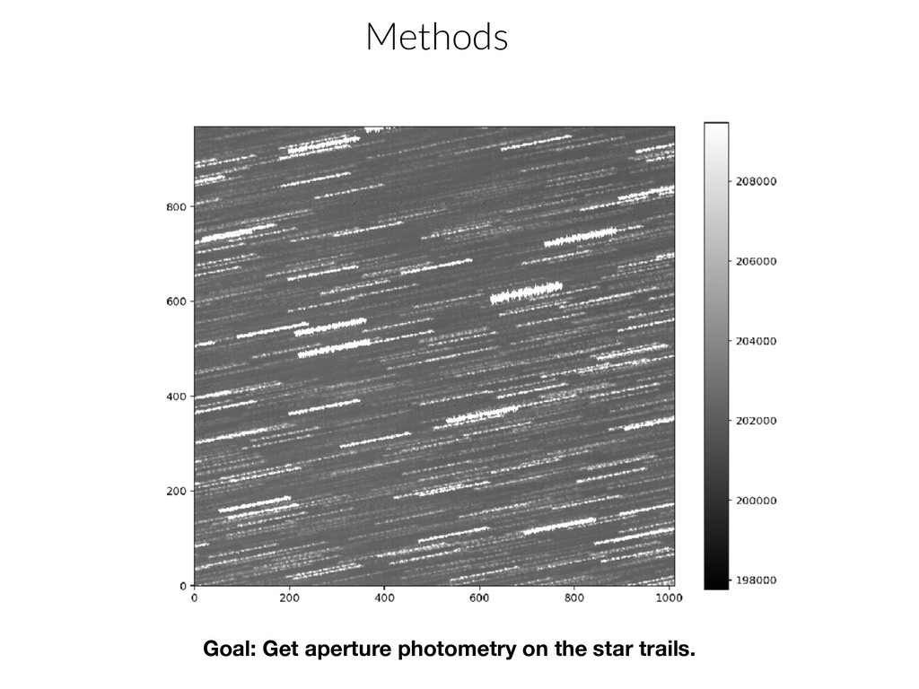
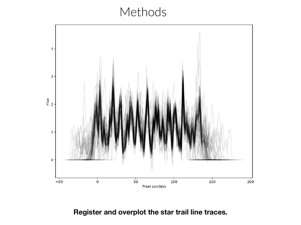
Driftscanning will produce long overlapping star-trails on the FFI, rather than conventional sharp point-sources. The star trails extend over ~150 +/- 20 pixels, corresponding to an average drift rate of ~0.35 arcseconds per second. The direction of pointing of the telescope was not known a-priori, but can in principle be derived from the distinct constellation pattern of star trails.

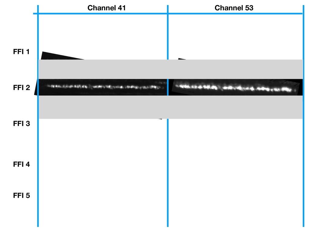
The driftscan FFIs were acquired with the same combined exposure time as conventional 30-minute Long Cadence FFIs, i.e. 270 onboard-coadded integrations with 6.02s exposure time and 0.52s readout time per integration. The DFFIs were collected within 16 minutes to 5 hours of the previous frame, such that star trails can be seen moving across module boundaries from frame-to-frame.

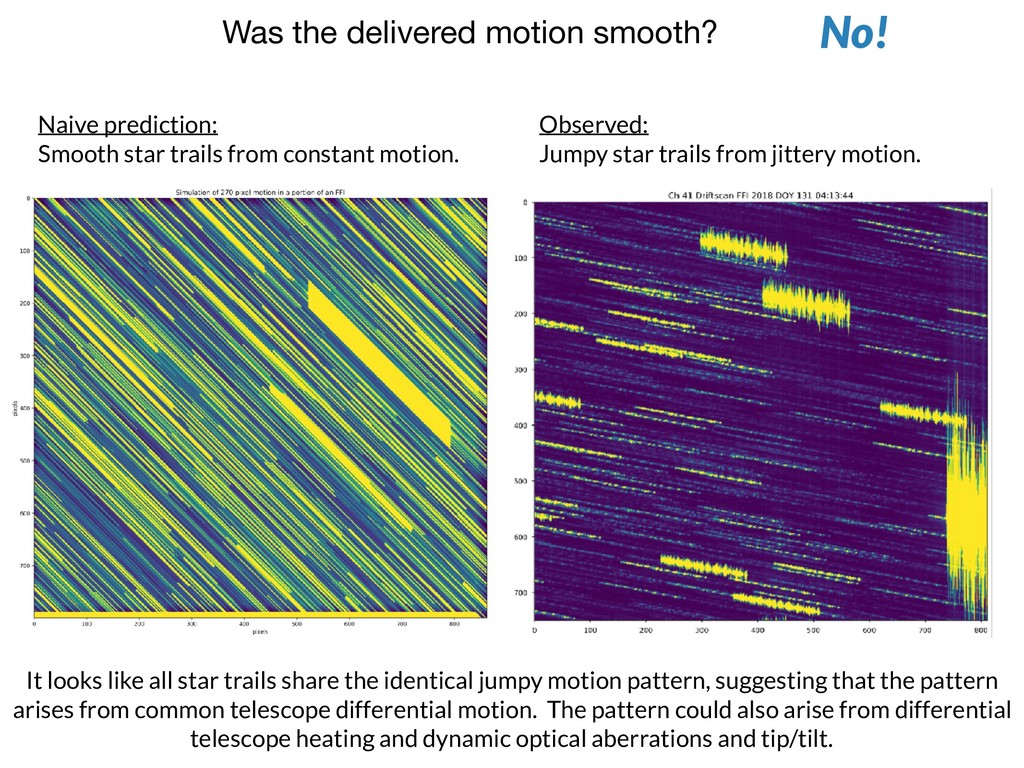
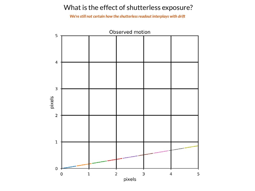
The star trail line segments possess substructure suggestive of non-constant image motion. A longer-than-average dwell time of a point source causes regions of "burn-in", while shorter-than-average dwell times cause relative dearths in flux. The resulting undulations appear in all the star trail line segments for a given driftscan FFI. The line segment substructures could also arise from the shutterless image array transfer process occurring in phase with constant image motion, yielding a "beating" phenomenon within pixel boundaries.

The driftscan FFIs may enhance flat-field calibration of the Kepler focal plane, since the relative response of adjacent pixels can be derived by identifying local departures from the expected star trail illumination pattern. Other uses for driftscan FFIs may eventually include solar system science and short-timescale (few seconds) variations of bright astrophysical sources.

This data should be considered experimental, and will not be pipeline-processed due to its irregular star trail patterns.
More information is available at https://keplerscience.arc.nasa.gov/

Transcript

1. Driftscan FFI analysis Michael Gully-Santiago Kepler/K2 GO Office May 14-15, 2018
2. Driftscanning is an experimental data collection mode in which the telescope collects a Full Frame Image (FFI) while the telescope is drifting in (TWSDDL). This animation simulates the data collection process with expected 0.5deg/hr. Only the final frame is telemetered back to Earth, yielding overlapping star trails.
3. Only the final frame is telemetered back to Earth, yielding overlapping star trails.
4. Motivation for FFI experiment 1. Pixel sensitivity calibration (flat field correction)
 2. Astrophysical variation on very short (~ten seconds) timescales
 3. Joint modeling of faint stars (e.g. Trappist-1) with underlying calibration (advanced)
5. 1. It doesn’t matter where you point.
 2. Delivers usable data over a wide range of angular motions (e.g. low-fuel conditions).
 3. Does not require any “heroic efforts”-- no new operational modes: just normal FFI sequence.
 4. Can be carried out during periods of extended indecision (TWSM, post-ARB but pre-TWSDDL).
 5. Avoids wasting precious pre-allocated DSN time.
 6. Has the potential to enhance all Kepler data ever taken, including from the prime mission. Operational advantages of driftscan FFIs 1. Not better than a regular science campaign.
 2. Data analysis will be unusual.
 3. Still costs DSN time that could have been allocated to other NASA missions.
 4. It’s not clear how pixel calibration changes in time (ask D. Caldwell about SPSDs). Operational limitations of driftscan FFIs
6. A short pilot program was carried out on May 10-11, 2018, to evaluate the feasibility of driftscan FFI operations. Driftscan FFIs were collected during the K2 Campaign 17 (C17) Deep Space Network (DSN) downlink, after all C17 science data had been safely telemetered and spare DSN time remained.
7. Anticipated questions (easy) 1.How many FFIs were taken? 2.What were the delay-times between acquisitions? 3.What was the delivered motion? 4.Was the motion primarily in (x,y), or was there rotation also? 5.Was the delivered motion smooth? 6.What is the distribution of S/N per pixel? 7.Did saturated stars ruin the exposures? 8.Can you associate star trails from one FFI with the next FFI?
8. Anticipated questions (harder) 9.Where was Kepler pointing during the exposures? 10.What was the stellar density? 11.What is the effect of shutterless exposure? 12.What was the angular acceleration of the telescope as a function of time? 13.Do you observe PSF variation? 14.Do you observe short-timescale astrophysical variability?
9. Anticipated questions (research project) 15.Is the variance of star trails consistent with flat field effects? 16.For what fraction of pixels do you have sufficient S/N to compute a revised flat field? 17.If that subset is finite, how does the revised flat field compare to the lab-measured flat field? 18.Do you observe chromatic-dependence in PSF variation?
10. How many FFIs were taken? What were the delay-times between acquisitions? kplr2018131024020_ffi-orig.fits kplr2018131032646_ffi-orig.fits kplr2018131041344_ffi-orig.fits kplr2018131094047_ffi-orig.fits kplr2018131130639_ffi-orig.fits Year DOY HH MM SS We took 5 FFIs. The exposure time is 30 minutes, so the delay between the end of one and beginning of the next ranges from 16 minutes to ~5 hours. The save to SSR command takes ~15 minutes. (Marcie Smith, Doug Caldwell priv. comm.) FFI num delay between (min) 1 0 2 16 3 17 4 297 5 176
11. What was the delivered motion? FFI num Channel length (pixels) motion (deg/hr) =("/sec) 1 41 155 0.350 1 53 152 0.346 2 41 157 0.356 2 53 156 0.354 3 41 158 0.359 3 53 157 0.357 4 41 144 0.326 4 53 141 0.319 5 41 156 0.353 5 53 153 0.347 The delivered motion was ~0.35 degrees/hour, slightly less than the coarse 0.5 degrees/hour prediction. The fourth FFI had about 10% slower motion than the others. ~150 pixels conversion factors 4"/pixel 29.4 minute exposure time
12. What was the delivered motion? FFI num Channel length (pixels) motion (deg/hr) =("/sec) 1 41 155 0.350 1 53 152 0.346 2 41 157 0.356 2 53 156 0.354 3 41 158 0.359 3 53 157 0.357 4 41 144 0.326 4 53 141 0.319 5 41 156 0.353 5 53 153 0.347 The delivered motion was ~0.35 degrees/hour, slightly less than the coarse 0.5 degrees/hour prediction. The fourth FFI had about 10% slower motion than the others.
13. Was the motion primarily in (x,y), or was there rotation also? The driftscan line segments look mostly like lines, not curved like sickles, suggesting that most of the motion was from linear telescope pointing drift, and not rotation around the boresight. The driftscan line segments have about the same length from center to edge. Channel 41, near the boresight center, possesses routinely longer line segments than Channel 53. This effect can be caused by either gradual rotation about an axis outside of the telescope FOV, or different PSF sizes, leading to biased line-segment estimation. straight lines curved lines not observed
14. Was the delivered motion smooth? No! Naive prediction: Smooth star trails from constant motion. Observed: Jumpy star trails from jittery motion. It looks like all star trails share the identical jumpy motion pattern, suggesting that the pattern arises from common telescope differential motion. The pattern could also arise from differential telescope heating and dynamic optical aberrations and tip/tilt.
15. What is the distribution of S/N per pixel? About 1.7% of pixels have S/N 100 or greater.
16. Did saturated stars ruin the exposures? No. Some streaking, but no irretrievable information loss Worry was that saturated stars in collateral smear data would make it impossible to determine the flux in pixels above or below the saturated stars.
17. Can you associate star trails from one FFI with the next FFI? Yes.
21. Answer to questions (easy) 1.How many FFIs were taken? 5 2.What were the delay-times between acquisitions? 16 min - 5 hrs 3.What was the delivered motion? ~0.35 deg/hr 4.Was the motion primarily in (x,y), or was there rotation also? primarily in (x,y) 5.Was the delivered motion smooth? No! 6.What is the distribution of S/N per pixel? ~1.7% of pixels have S/N 100 or more 7.Did saturated stars ruin the exposures? No. 8.Can you associate star trails from one FFI with the next FFI? Yes.
22. Anticipated questions (harder) 9.Where was Kepler pointing during the exposures? TBD... 10.What was the stellar density? TBD... 11.What is the effect of shutterless exposure? TBD, see Next slide 12.What was the angular acceleration of the telescope as a function of time? Next slide + 1 13.Do you observe PSF variation? TBD... 14.Do you observe short-timescale astrophysical variability? TBD...
23. What is the effect of shutterless exposure? We're still not certain how the shutterless readout interplays with drift
24. What was the angular acceleration of the telescope as a function of time?
25. Methods Goal: Get aperture photometry on the star trails.
26. Methods Assemble a convolution kernel from a high S/N, unsaturated, isolated, filtered star trail.
27. Methods Perform source extraction using the convolution kernel. Reject saturated and partial trails
28. Methods Perform custom aperture photometry on each source. Many sources overlap with adjacent star trails.
29. Methods Register and overplot the star trail line traces.
30. Channel 41 Channel 53 FFI 1 FFI 2 FFI 3 FFI 4 FFI 5