Frontiers in forward modeling substellar atmospheres

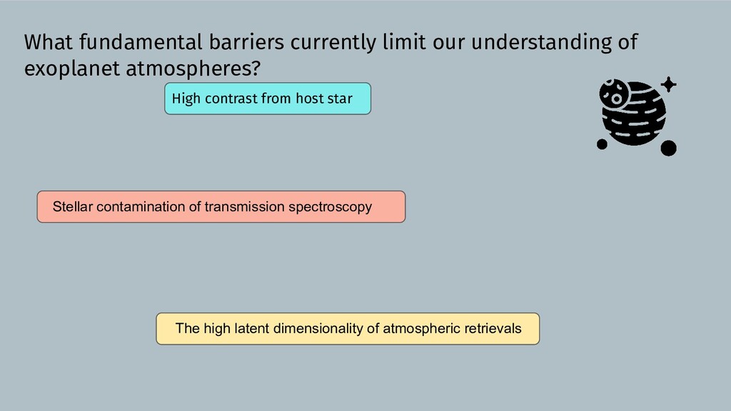
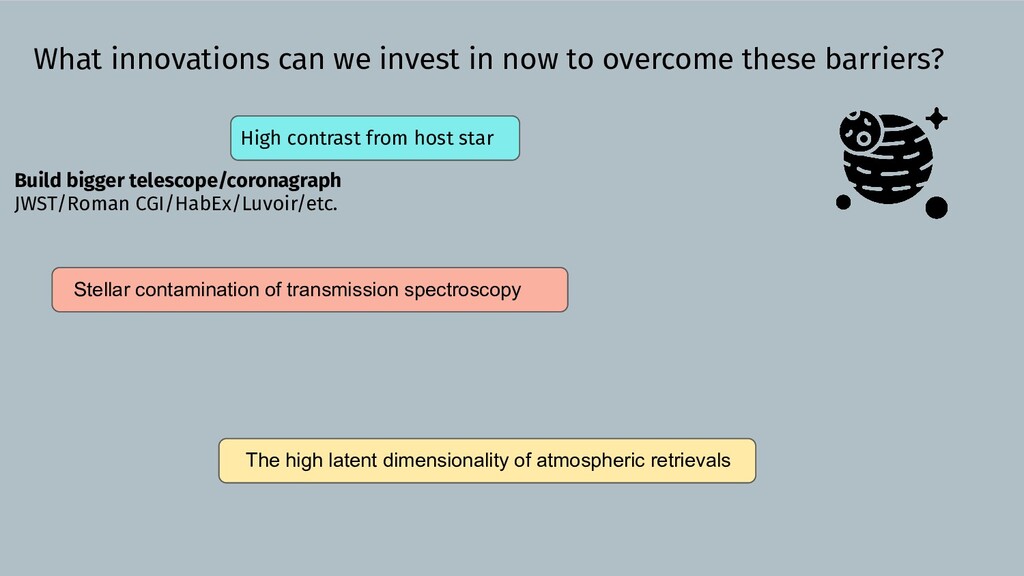
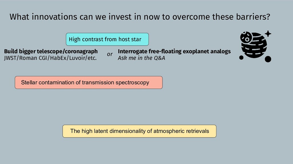
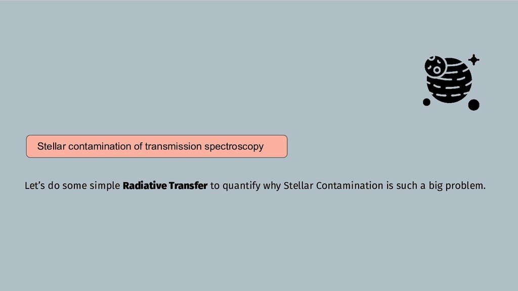
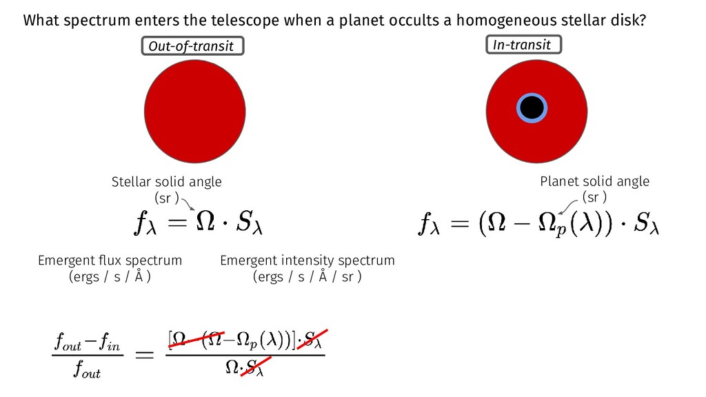
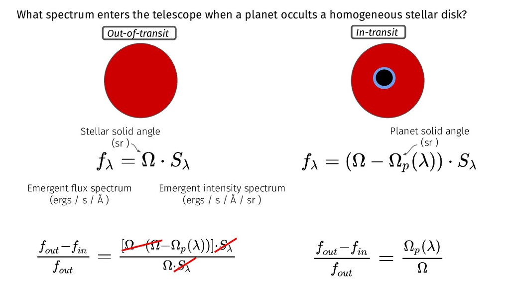
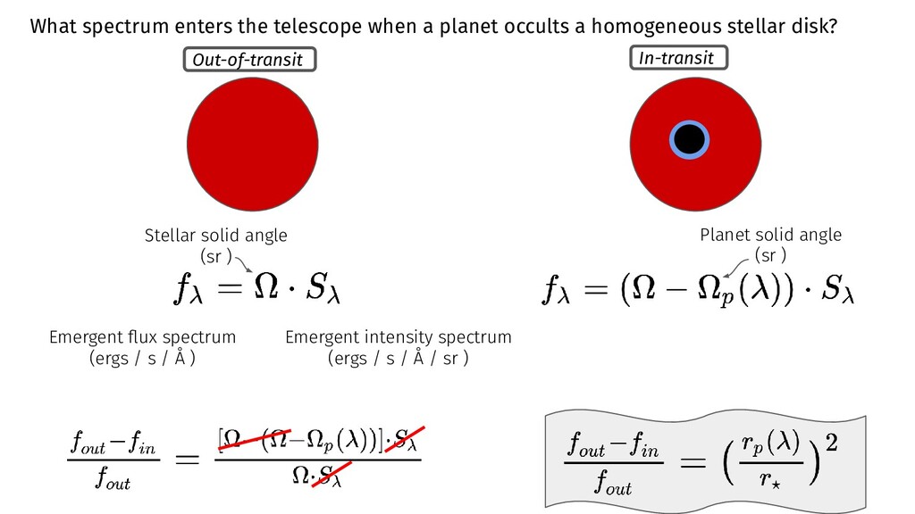
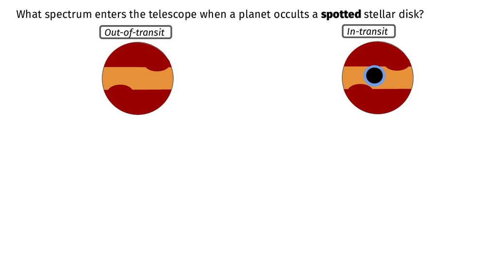
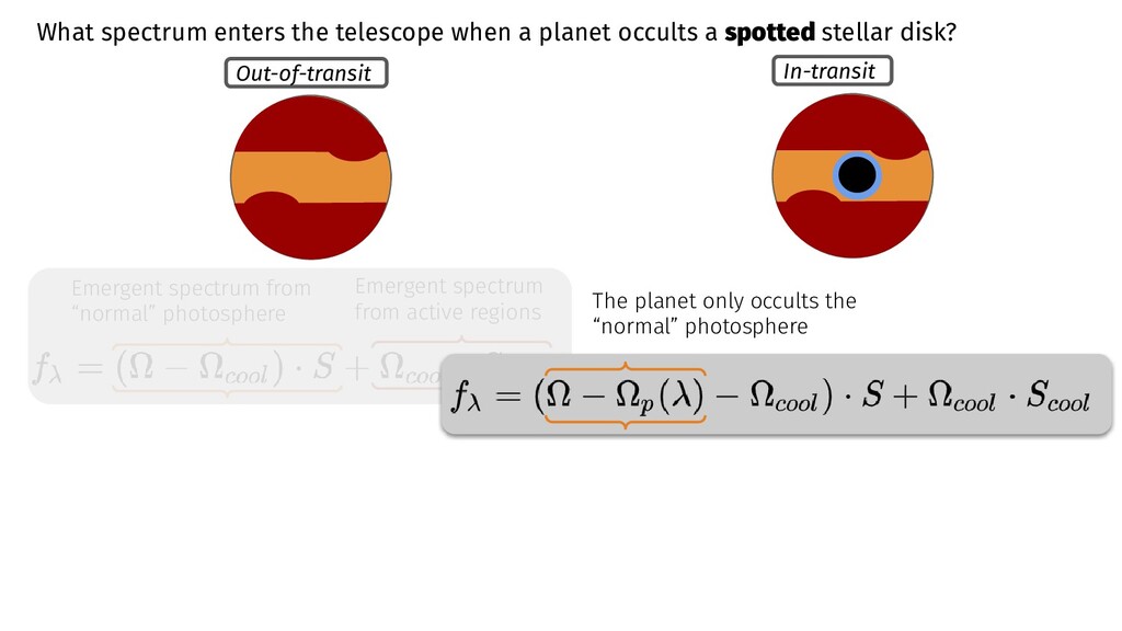
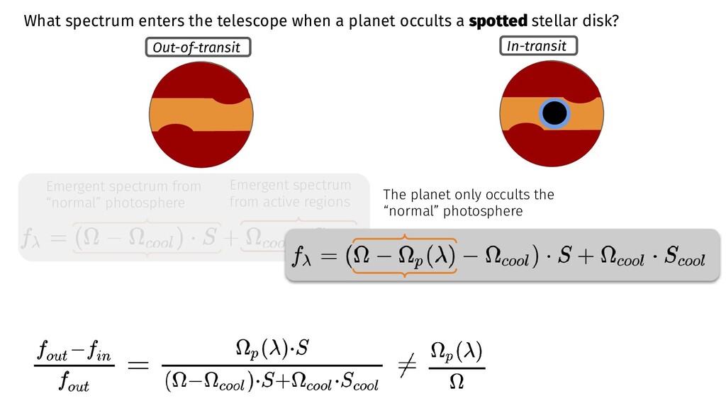
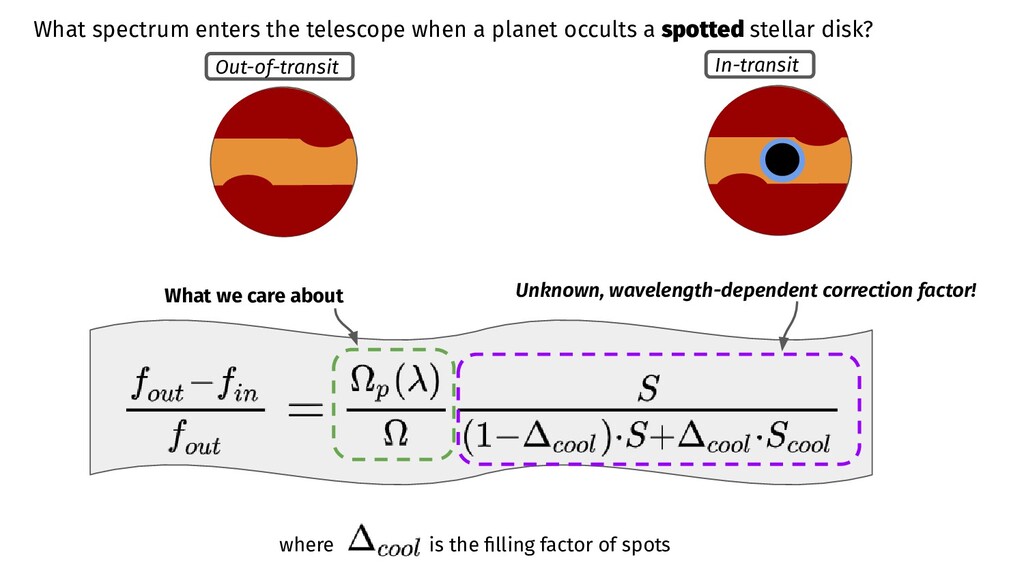
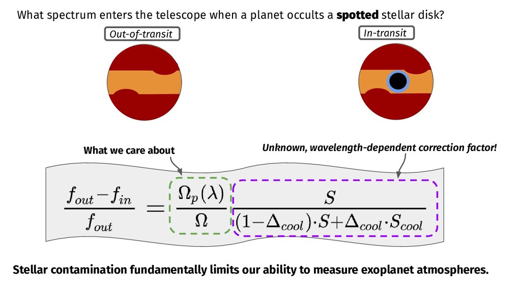
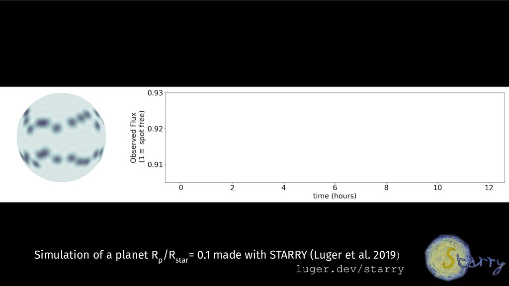
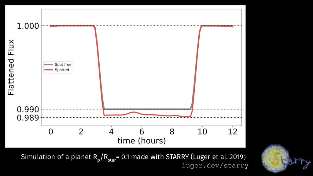
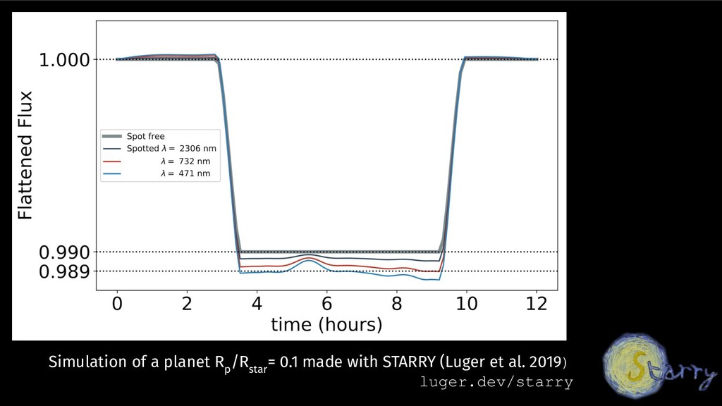
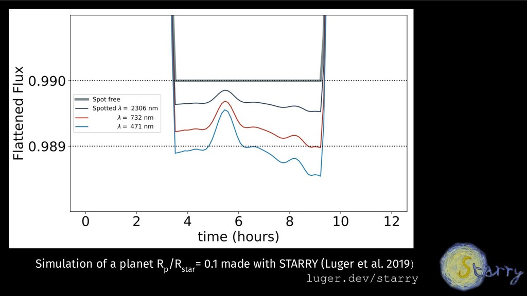
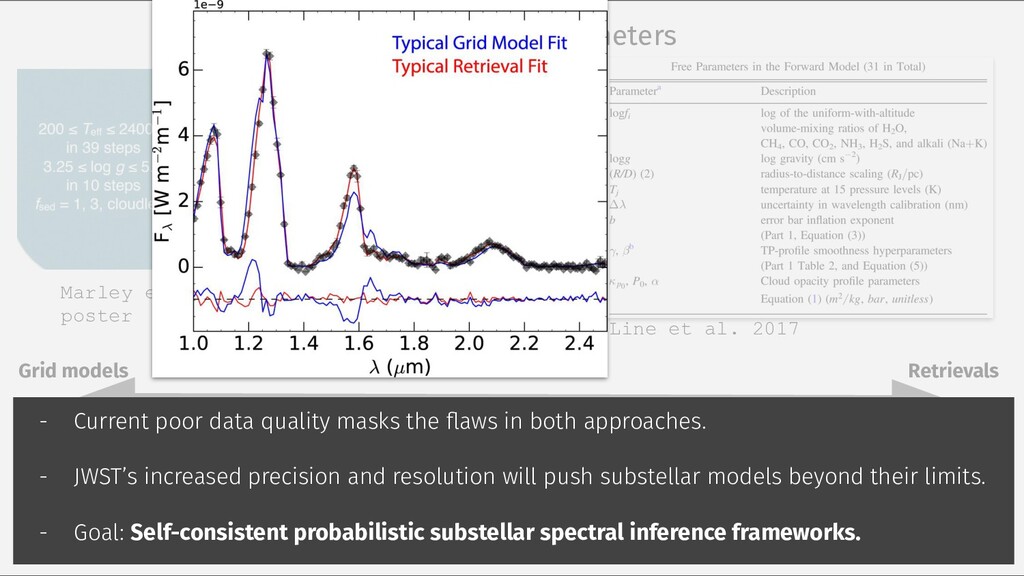
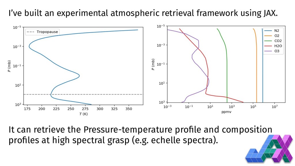
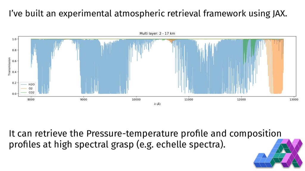
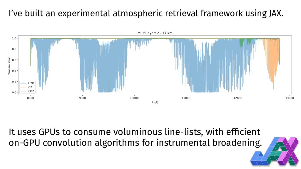
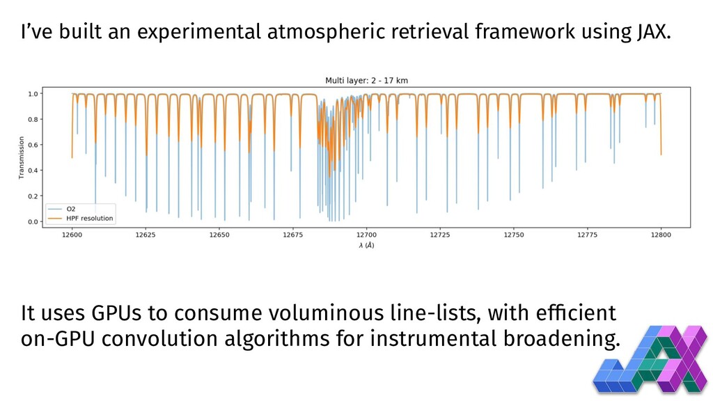
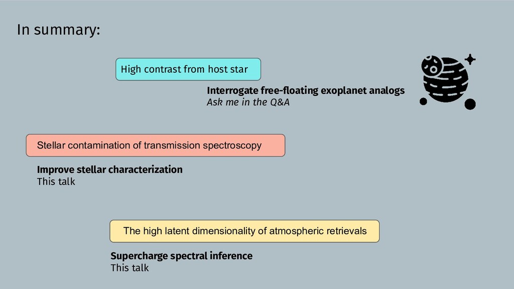
Three fundamental barriers currently limit our understanding of exoplanet atmospheres. High contrast from exoplanet host stars, stellar contamination in transmission spectroscopy, and the high dimensionality of atmospheric retrievals all ultimately hamper investigations of exoplanetary habitability. In this talk I quantify the size of the confounding effects and show experimental progress we have made in overcoming these challenges. Our solutions employ probabilistic spectral inference to account for inherent degeneracies in extracting weak signals from astronomical spectra.

This 25 minute talk was given remotely at the weekly "Stars, Planets, and ISM Seminar" at The University of Texas at Austin Department of Astronomy on October 7, 2020. A screencast recording exists and may be made available upon request.

Transcript

1. Frontiers in forward modeling substellar atmospheres Michael Gully-Santiago Research Fellow UT Austin Department of Astronomy Stars/Planets/ISM Seminar October 7, 2020
2. What fundamental barriers currently limit our understanding of exoplanet atmospheres?
3. What fundamental barriers currently limit our understanding of exoplanet atmospheres? Stellar contamination of transmission spectroscopy High contrast from host star The high latent dimensionality of atmospheric retrievals
4. What innovations can we invest in now to overcome these barriers? Stellar contamination of transmission spectroscopy The high latent dimensionality of atmospheric retrievals Build bigger telescope/coronagraph JWST/Roman CGI/HabEx/Luvoir/etc. High contrast from host star
5. What innovations can we invest in now to overcome these barriers? Stellar contamination of transmission spectroscopy The high latent dimensionality of atmospheric retrievals Build bigger telescope/coronagraph JWST/Roman CGI/HabEx/Luvoir/etc. Interrogate free-floating exoplanet analogs Ask me in the Q&A or High contrast from host star
6. What innovations can we invest in now to overcome these barriers? Stellar contamination of transmission spectroscopy The high latent dimensionality of atmospheric retrievals Build bigger telescope/coronagraph JWST/Roman CGI/HabEx/Luvoir/etc. Improve stellar characterization This talk Interrogate free-floating exoplanet analogs Ask me in the Q&A or High contrast from host star
7. What innovations can we invest in now to overcome these barriers? Stellar contamination of transmission spectroscopy The high latent dimensionality of atmospheric retrievals Build bigger telescope/coronagraph JWST/Roman CGI/HabEx/Luvoir/etc. Improve stellar characterization This talk Supercharge spectral inference This talk Interrogate free-floating exoplanet analogs Ask me in the Q&A or High contrast from host star
8. Stellar contamination of transmission spectroscopy Let’s do some simple Radiative Transfer to quantify why Stellar Contamination is such a big problem.
9. What spectrum enters the telescope when a planet occults a homogeneous stellar disk? Emergent flux spectrum (ergs / s / Å ) Emergent intensity spectrum (ergs / s / Å / sr ) Stellar solid angle (sr ) Out-of-transit In-transit
10. What spectrum enters the telescope when a planet occults a homogeneous stellar disk? Emergent flux spectrum (ergs / s / Å ) Emergent intensity spectrum (ergs / s / Å / sr ) Stellar solid angle (sr ) Planet solid angle (sr ) Out-of-transit In-transit
11. What spectrum enters the telescope when a planet occults a homogeneous stellar disk? Emergent flux spectrum (ergs / s / Å ) Emergent intensity spectrum (ergs / s / Å / sr ) Stellar solid angle (sr ) Planet solid angle (sr ) Out-of-transit In-transit
12. What spectrum enters the telescope when a planet occults a homogeneous stellar disk? Emergent flux spectrum (ergs / s / Å ) Emergent intensity spectrum (ergs / s / Å / sr ) Stellar solid angle (sr ) Planet solid angle (sr ) Out-of-transit In-transit
13. What spectrum enters the telescope when a planet occults a homogeneous stellar disk? Emergent flux spectrum (ergs / s / Å ) Emergent intensity spectrum (ergs / s / Å / sr ) Stellar solid angle (sr ) Planet solid angle (sr ) Out-of-transit In-transit
14. What spectrum enters the telescope when a planet occults a homogeneous stellar disk? Emergent flux spectrum (ergs / s / Å ) Emergent intensity spectrum (ergs / s / Å / sr ) Stellar solid angle (sr ) Planet solid angle (sr ) Out-of-transit In-transit
15. What spectrum enters the telescope when a planet occults a homogeneous stellar disk? Emergent flux spectrum (ergs / s / Å ) Emergent intensity spectrum (ergs / s / Å / sr ) Stellar solid angle (sr ) Planet solid angle (sr ) Out-of-transit In-transit
16. What spectrum enters the telescope when a planet occults a spotted stellar disk? Out-of-transit In-transit
17. Out-of-transit In-transit What spectrum enters the telescope when a planet occults a spotted stellar disk?
18. Out-of-transit In-transit What spectrum enters the telescope when a planet occults a spotted stellar disk? Emergent spectrum from “normal” photosphere Emergent spectrum from active regions
19. Out-of-transit In-transit What spectrum enters the telescope when a planet occults a spotted stellar disk? Emergent spectrum from “normal” photosphere Emergent spectrum from active regions
20. Out-of-transit In-transit What spectrum enters the telescope when a planet occults a spotted stellar disk? Emergent spectrum from “normal” photosphere Emergent spectrum from active regions
21. Out-of-transit In-transit What spectrum enters the telescope when a planet occults a spotted stellar disk? Emergent spectrum from “normal” photosphere Emergent spectrum from active regions The planet only occults the “normal” photosphere
22. Out-of-transit In-transit What spectrum enters the telescope when a planet occults a spotted stellar disk? Emergent spectrum from “normal” photosphere Emergent spectrum from active regions The planet only occults the active region
23. Out-of-transit In-transit What spectrum enters the telescope when a planet occults a spotted stellar disk? Emergent spectrum from “normal” photosphere Emergent spectrum from active regions The planet only occults the “normal” photosphere
24. Out-of-transit In-transit What spectrum enters the telescope when a planet occults a spotted stellar disk? Emergent spectrum from “normal” photosphere Emergent spectrum from active regions The planet only occults the “normal” photosphere
25. Out-of-transit In-transit What spectrum enters the telescope when a planet occults a spotted stellar disk? where is the filling factor of spots What we care about Unknown, wavelength-dependent correction factor!
26. Out-of-transit In-transit What spectrum enters the telescope when a planet occults a spotted stellar disk? What we care about Stellar contamination fundamentally limits our ability to measure exoplanet atmospheres. Unknown, wavelength-dependent correction factor!
27. Simulation of a planet R p /R star = 0.1 made with STARRY (Luger et al. 2019) luger.dev/starry
28. Simulation of a planet R p /R star = 0.1 made with STARRY (Luger et al. 2019) luger.dev/starry
29. Simulation of a planet R p /R star = 0.1 made with STARRY (Luger et al. 2019) luger.dev/starry
30. Simulation of a planet R p /R star = 0.1 made with STARRY (Luger et al. 2019) luger.dev/starry
31. Simulation of a planet R p /R star = 0.1 made with STARRY (Luger et al. 2019) luger.dev/starry
32. Simulation of a planet R p /R star = 0.1 made with STARRY (Luger et al. 2019) luger.dev/starry Artificial water features appear in your spectrum
33. What are my collaborators and I doing to overcome stellar contamination? - Combined Kepler/K2 and IGRINS to measure the filling factor and spectrum of starspots on weak-lined Class III T-Tauri stars. (Gully-Santiago et al. 2017; prev. ISM talk) - Simulated impact of starspot geometry on lightcurves for a Pleiades-age population (Guo, Gully-Santiago, Herczeg 2018) - Expanding our starspot program to Gaia-DR2-selected underluminous sub-giants (Gosnell et al. in prep; ongoing w/Tofflemire IGRINS 2020B, 2.7 m, LCOGT NRES) - Monitoring heavily spotted TESS Cycle-1 selected Nearby Young Moving Group members (2021A IGRINS Band 3 Compensatory Time) - Experimental programs on heavily spotted exoplanet host stars (c.f. DS Tuc, Montet et al. 2020)
34. What are my collaborators and I doing to overcome stellar contamination? - Combined Kepler/K2 and IGRINS to measure the filling factor and spectrum of starspots on weak-lined Class III T-Tauri stars. (Gully-Santiago et al. 2017; prev. ISM talk) - Simulated impact of starspot geometry on lightcurves for a Pleiades-age population (Guo, Gully-Santiago, Herczeg 2018) - Expanding our starspot program to Gaia-DR2-selected underluminous sub-giants (Gosnell et al. in prep; ongoing w/Tofflemire IGRINS 2020B, 2.7 m, LCOGT NRES) - Monitoring heavily spotted TESS Cycle-1 selected Nearby Young Moving Group members (2021A IGRINS Band 3 Compensatory Time) - Experimental programs on heavily spotted exoplanet host stars (c.f. DS Tuc, Montet et al. 2020)
35. What are my collaborators and I doing to overcome stellar contamination? - Combined Kepler/K2 and IGRINS to measure the filling factor and spectrum of starspots on weak-lined Class III T-Tauri stars. (Gully-Santiago et al. 2017; prev. ISM talk) - Simulated impact of starspot geometry on lightcurves for a Pleiades-age population (Guo, Gully-Santiago, Herczeg 2018) - Expanding our starspot program to Gaia-DR2-selected underluminous sub-giants (Gosnell et al. in prep; ongoing w/Tofflemire IGRINS 2020B, 2.7 m, LCOGT NRES) - Monitoring heavily spotted TESS Cycle-1 selected Nearby Young Moving Group members (2021A IGRINS Band 3 Compensatory Time) - Experimental programs on heavily spotted exoplanet host stars (c.f. DS Tuc, Montet et al. 2020)
36. What are my collaborators and I doing to overcome stellar contamination? - Combined Kepler/K2 and IGRINS to measure the filling factor and spectrum of starspots on weak-lined Class III T-Tauri stars. (Gully-Santiago et al. 2017; prev. ISM talk) - Simulated impact of starspot geometry on lightcurves for a Pleiades-age population (Guo, Gully-Santiago, Herczeg 2018) - Expanding our starspot program to Gaia-DR2-selected underluminous sub-giants (Gosnell et al. in prep; ongoing w/Tofflemire IGRINS 2020B, 2.7 m, LCOGT NRES) - Monitoring heavily spotted TESS Cycle-1 selected Nearby Young Moving Group members (2021A IGRINS Band 3 Compensatory Time) - Experimental programs on heavily spotted exoplanet host stars (c.f. DS Tuc, Montet et al. 2020)
37. What are my collaborators and I doing to overcome stellar contamination? - Combined Kepler/K2 and IGRINS to measure the filling factor and spectrum of starspots on weak-lined Class III T-Tauri stars. (Gully-Santiago et al. 2017; prev. ISM talk) - Simulated impact of starspot geometry on lightcurves for a Pleiades-age population (Guo, Gully-Santiago, Herczeg 2018) - Expanding our starspot program to Gaia-DR2-selected underluminous sub-giants (Gosnell et al. in prep; ongoing w/Tofflemire IGRINS 2020B, 2.7 m, LCOGT NRES) - Monitoring heavily spotted TESS Cycle-1 selected Nearby Young Moving Group members (2021A IGRINS Band 3 Compensatory Time) - Experimental programs on heavily spotted exoplanet host stars (c.f. DS Tuc, Montet et al. 2020)
38. What is the future of these programs at UTexas? What’s conceivable? - Stellar characterization of Helium Exospheres sample, deep dive on chromospheric lines - TESS Cycle 4, not yet announced but likely to visit the ecliptic plane: quantify spot contrast with K2 and TESS amplitudes head-to-head - Contemporaneous TESS observations with HPF in HET 2020-2 & 2020-3 - Apply probabilistic Doppler Imaging framework Paparazzi (Luger et al. in prep) to HPF spectra for velocity-resolved-decomposition - HST Archival Program to assess stellar contamination in extant data
39. What is the future of these programs at UTexas? What’s conceivable? - Stellar characterization of Helium Exospheres sample, deep dive on chromospheric lines - TESS Cycle 4, not yet announced but likely to visit the ecliptic plane: quantify spot contrast with K2 and TESS amplitudes head-to-head - Contemporaneous TESS observations with HPF in HET 2020-2 & 2020-3 - Apply probabilistic Doppler Imaging framework Paparazzi (Luger et al. in prep) to HPF spectra for velocity-resolved-decomposition - HST Archival Program to assess stellar contamination in extant data Luger et al. in prep
40. The high latent dimensionality of atmospheric retrievals Supercharge spectral inference
41. How many free parameters does a substellar atmosphere have?
42. How many free parameters does a substellar atmosphere have? Practically speaking, which and how many parameters should I include when building a forward model of a substellar atmosphere? What sets the limit? Along how many axes does nature produce observably distinct outcomes in the star/planet-formation lifecycle when observed at a range of snapshots in time?
43. Answer: ~4 - 31 free parameters Model flexibility axis Less flexible: ~4 parameters Physically self-consistent ~hour per spectrum Supports high spectral resolution Grid models Retrievals Marley et al. 2017 AAS poster More flexible: ~30 parameters Physically inconsistent ~second per spectrum Limited to low spectral resolution Line et al. 2017
44. A: ~4 - 31 free parameters Model flexibility axis Less flexible: ~4 parameters Physically self-consistent ~hour per spectrum Supports high spectral resolution Grid models Retrievals Marley et al. 2017 AAS poster More flexible: ~30 parameters Physically inconsistent ~second per spectrum Limited to low spectral resolution Line et al. 2017 - Current poor data quality masks the flaws in both approaches. - JWST’s increased precision and resolution will push substellar models beyond their limits. - Goal: Self-consistent probabilistic substellar spectral inference frameworks.
45. Starfish: Self-consistent probabilistic spectral inference with grid models Starfish provides a flexible likelihood function for grid models through several computational and statistical breakthroughs (Czekala et al. 2015) I have extended the framework to the new Sonora models, making it possible to do probabilistic inference on high-resolution spectra of ultracool L and T dwarfs with IGRINS, Keck-NIRSPEC, and HPF. U Hawaii Graduate Student ZJ Zhang has based much of his PhD thesis on this foundation. github.com/gully/jammer-Gl570D ^Watch my SciPy 2020 talk on YouTube: Applying Probabilistic Inference to Astronomical Spectroscopy
46. A deep dive on modern computational astrophysics intended to illuminate the path towards JWST-era-and-beyond retrievals of substellar and exoplanet atmospheres.
47. My Sonora-adapted Starfish and Mike Line’s retrieval code Chimera both use emcee. With almost 4000 citations since 2013, it is one of the most cited papers in all of modern astrophysics.
48. Most likely, you, or your graduate students advisees, or your collaborators have used emcee. emcee’s popularity stems from its high-performance, ease-of-use, abundant tutorials, ability to parallelize on modern CPUs, and other factors*. But emcee’s ensemble algorithm fundamentally limits how many parameters you can have in your model. *See speakerdeck.com/dfm/emcee-odi for lessons learned from emcee.
49. statmodeling.stat.columbia.edu/2017/03/15/ensemble-methods-doomed-fail-high-dimensions/
50. 25 parameters means exploring a 25 dimensional space - Red contours show true independent samples from a 25-dimensional correlated multivariate normal distribution - Blue contours show emcee random walk exploration of this hypervolume.
51. 300 parameters means exploring a 300 dimensional space - Blue contours show true independent samples from a 300-dimensional correlated multivariate normal distribution - Red contours show emcee random walk exploration of this hypervolume.
52. 300 parameters means exploring a 300 dimensional space - Blue contours show true independent samples from a 300-dimensional correlated multivariate normal distribution - Red contours show emcee random walk exploration of this hypervolume.
54. Take derivatives? Of what? Why derivatives?
55. “Hamiltonian Monte Carlo (HMC) is a Markov chain Monte Carlo (MCMC) algorithm that avoids the random walk behavior and sensitivity to correlated parameters that plague many MCMC methods by taking a series of steps informed by first-order gradient information.” Hoffman & Gelman 2011 Betancourt 2016
56. “Hamiltonian Monte Carlo (HMC) is a Markov chain Monte Carlo (MCMC) algorithm that avoids the random walk behavior and sensitivity to correlated parameters that plague many MCMC methods by taking a series of steps informed by first-order gradient information.” Hoffman & Gelman 2011 Betancourt 2016 If you can take the derivative of your likelihood function, you can treat your atmospheric retrieval as running a Hamiltonian dynamics simulation.
57. 300 parameters means exploring a 300 dimensional space - Blue contours show true independent samples from a 300-dimensional correlated multivariate normal distribution - Red contours show emcee random walk exploration of this hypervolume.
58. 300 parameters means exploring a 300 dimensional space - Blue contours show true independent samples from a 300-dimensional correlated multivariate normal distribution - Red contours show Hamiltonian Monte Carlo random walk exploration of this hypervolume. Much faster convergence in high dimensions
59. How do you take derivatives of your likelihood function??
60. How do you take derivatives of your likelihood function?? What foundations have made machine learning / AI so successful in industrial applications? - Vast amounts of data - High-throughput computing (GPUs/TPUs) - Neural architectures - Automatic differentiation (of loss functions)
61. How do you take derivatives of your likelihood function?? What foundations have made machine learning / AI so successful in industrial applications? - Vast amounts of data - High-throughput computing (GPUs/TPUs) - Neural architectures - Automatic differentiation (of loss functions)
62. Modern machine learning frameworks enable you to take the derivative of scalar loss functions, e.g. chi-squared.
63. Modern machine learning frameworks enable you to take the derivative of scalar loss functions, e.g. chi-squared. One new framework allows you to take derivatives of any* function.
64. I’ve built an experimental atmospheric retrieval framework using JAX. It can retrieve the Pressure-temperature profile and composition profiles at high spectral grasp (e.g. echelle spectra).
65. I’ve built an experimental atmospheric retrieval framework using JAX. It can retrieve the Pressure-temperature profile and composition profiles at high spectral grasp (e.g. echelle spectra).
66. I’ve built an experimental atmospheric retrieval framework using JAX. It uses GPUs to consume voluminous line-lists, with efficient on-GPU convolution algorithms for instrumental broadening.
67. I’ve built an experimental atmospheric retrieval framework using JAX. It uses GPUs to consume voluminous line-lists, with efficient on-GPU convolution algorithms for instrumental broadening.
68. I’ve built an experimental atmospheric retrieval framework using JAX. It can take exact derivatives of your spectrum with-respect-to all parameters (i.e. the Jacobian), for free.
69. I’ve built an experimental atmospheric retrieval framework using JAX. It can take exact second derivatives of your spectrum with-respect-to all pairs of parameters (i.e. the Hessian)
70. I’ve built an experimental atmospheric retrieval framework using JAX. It works seamlessly with Hamiltonian Monte Carlo with hundreds or (eventually, with TACC?) thousands of free parameters.
71. I’ve built an experimental atmospheric retrieval framework using JAX. It is open source, in the form of Jupyter Notebook tutorials. github.com/BrownDwarf/fiatlux
72. In summary: Stellar contamination of transmission spectroscopy The high latent dimensionality of atmospheric retrievals Improve stellar characterization This talk Supercharge spectral inference This talk Interrogate free-floating exoplanet analogs Ask me in the Q&A High contrast from host star