This is the presentation for my Master Thesis for the MSc in Mathematics at Utrecht University. I present ideas for the extension of the medium-grain method for sparse matrix partitioning.
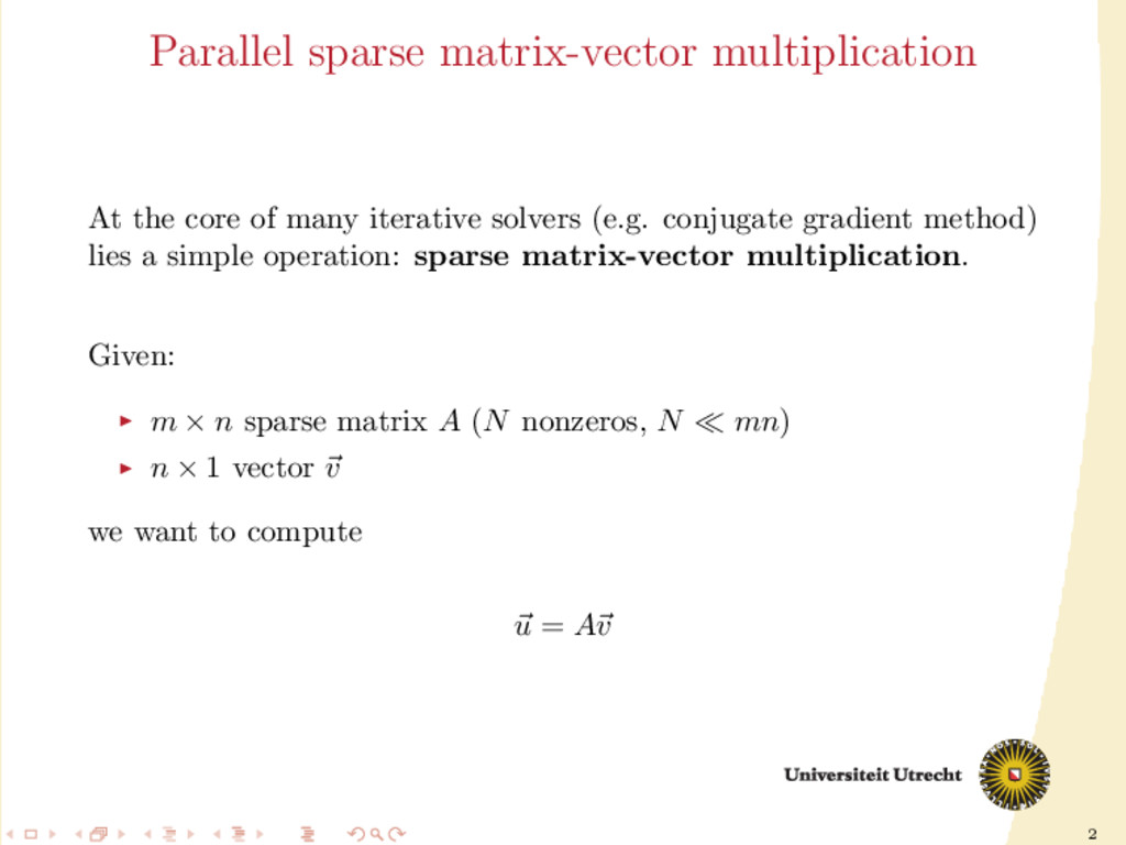
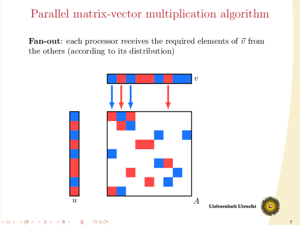
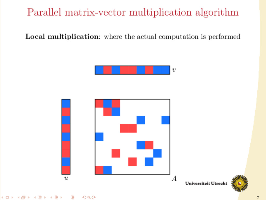
iterative solvers (e.g. conjugate gradient method) lies a simple operation: sparse matrix-vector multiplication. Given: m × n sparse matrix A (N nonzeros, N mn) n × 1 vector v we want to compute u = Av
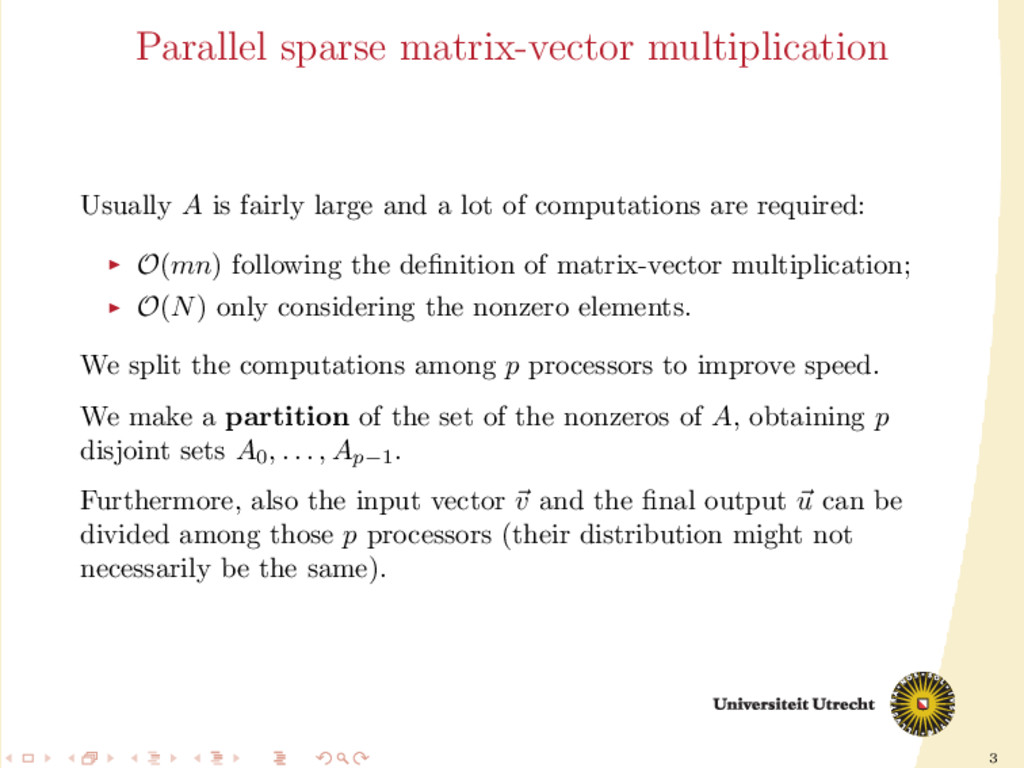
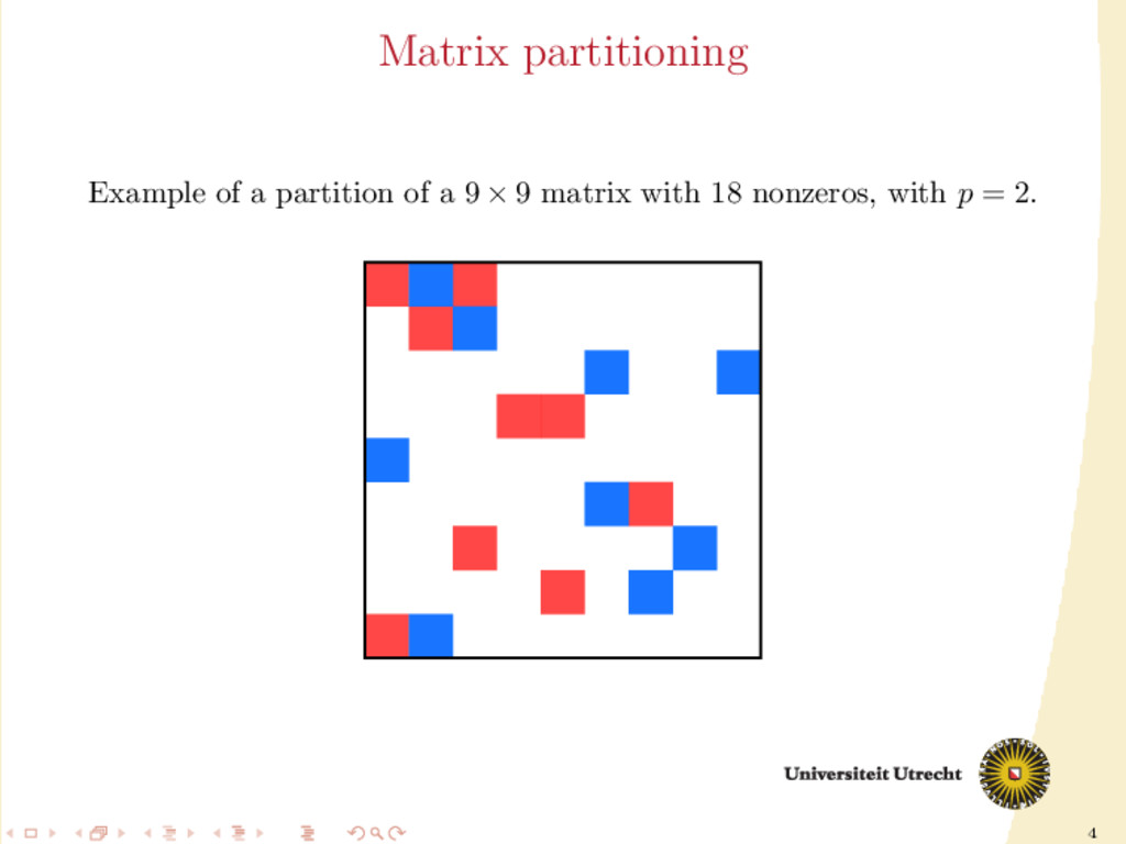
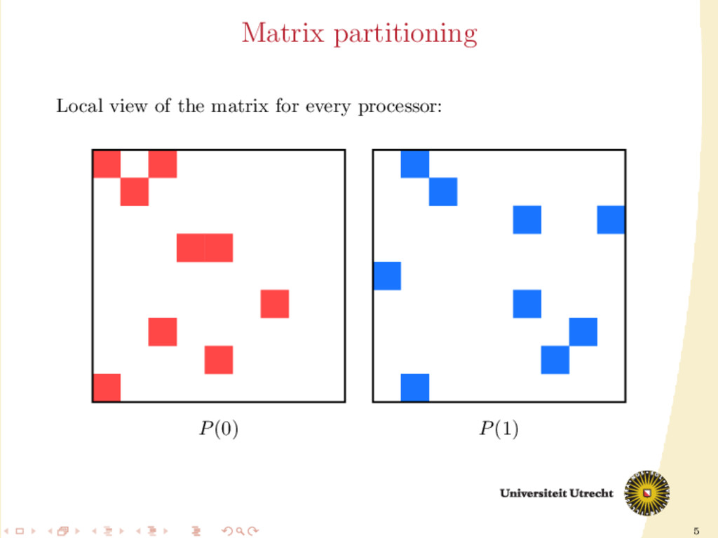
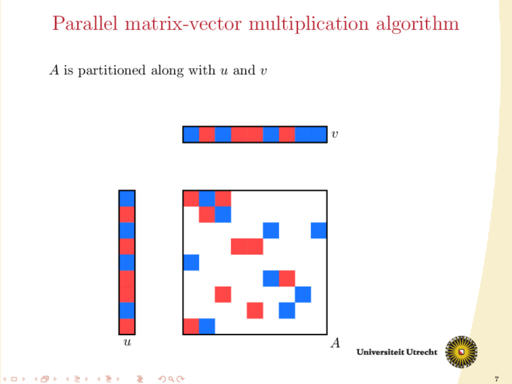
and a lot of computations are required: O(mn) following the definition of matrix-vector multiplication; O(N) only considering the nonzero elements. We split the computations among p processors to improve speed. We make a partition of the set of the nonzeros of A, obtaining p disjoint sets A0 , . . . , Ap−1 . Furthermore, also the input vector v and the final output u can be divided among those p processors (their distribution might not necessarily be the same).
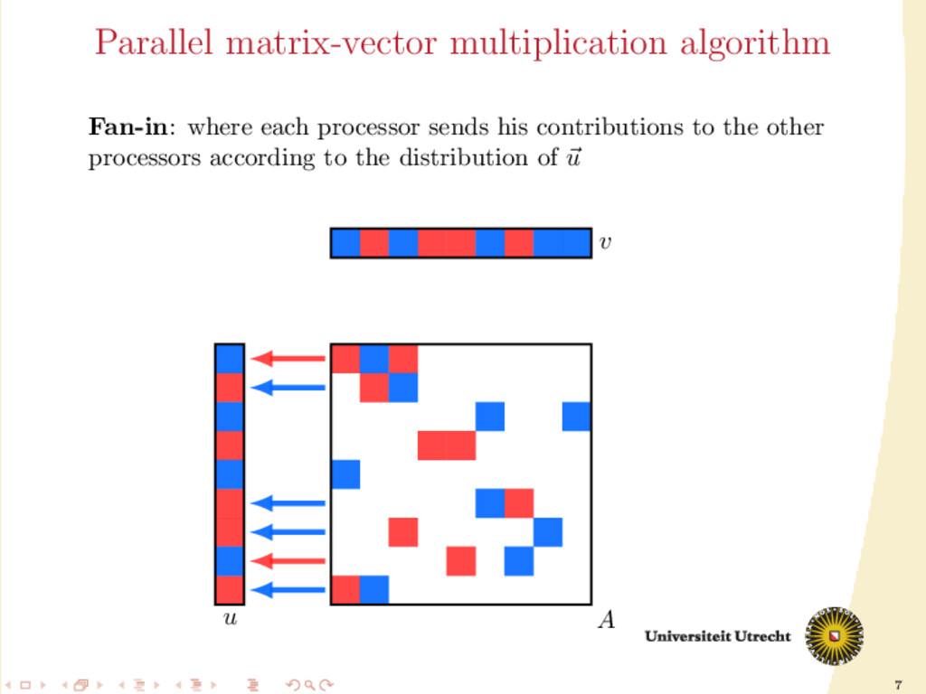
involve communication: it has to be minimized II is a computation step: we need balance in the size of the partitions Optimization problem: partition the nonzeros such that the balance constraint is satisfied and the communication volume is minimized.
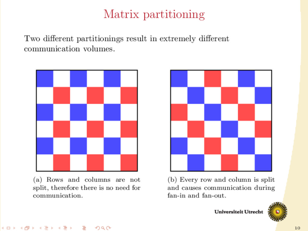
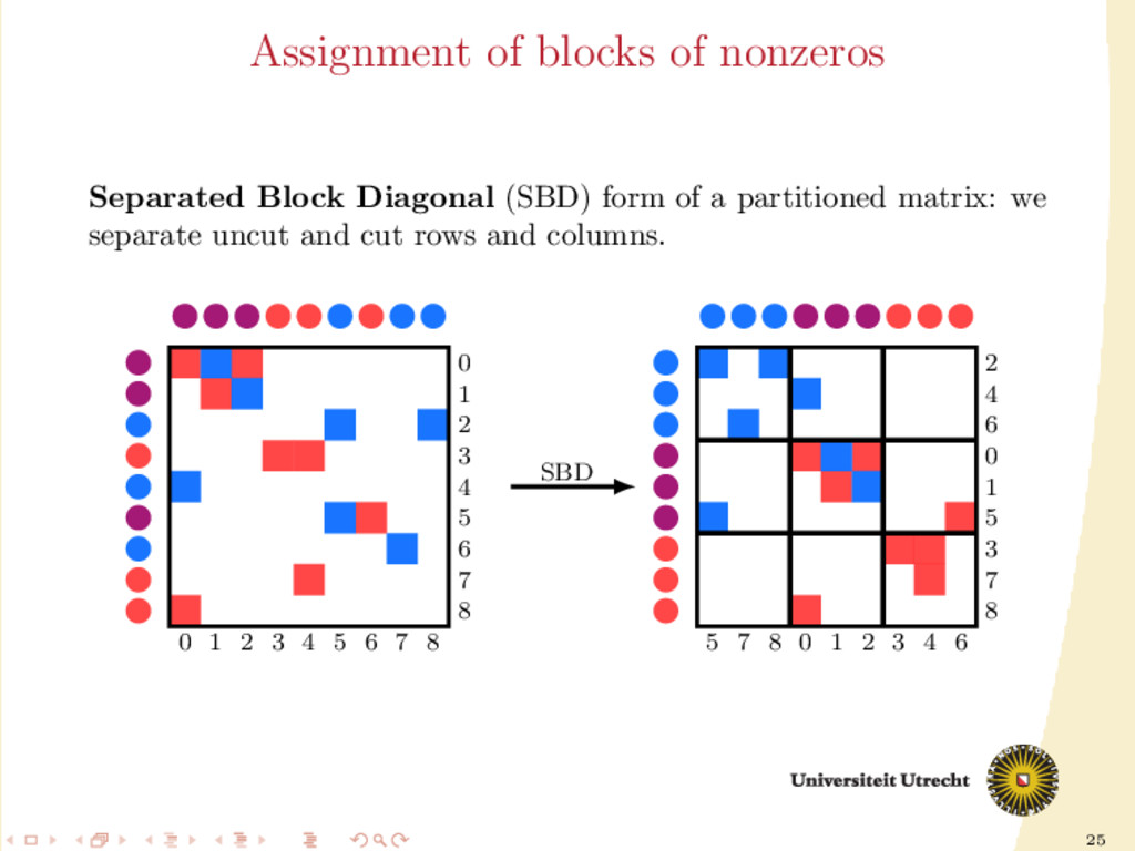
communication volumes. (a) Rows and columns are not split, therefore there is no need for communication. (b) Every row and column is split and causes communication during fan-in and fan-out.
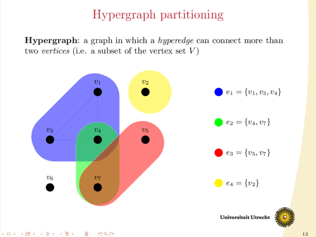
through hypergraph partitioning. A partition of a hypergraph is simply the partition of the set of vertices V into V0 , . . . , Vp−1 . A hyperedge e = {v1 , . . . , vk } is cut if two of its vertices belong to different sets of the partition.
matrix partitioning to hypergraph partitioning: 1-dimensional row-net: each column of A is a vertex in the hypergraph, each row a hyperedge. If aij = 0, then column Ai is placed in the hyperedge j. column-net: identical to the previous one, with the roles of columns and rows exchanged As hypergraph partitioning consists in assignment of the vertices, columns/rows are uncut. Advantage of eliminating completely one source of communication, but being 1-dimensional is often a too strong restriction.
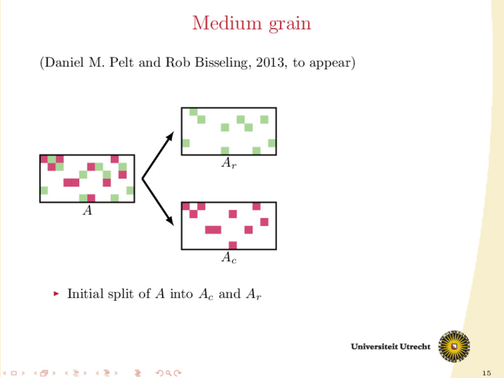
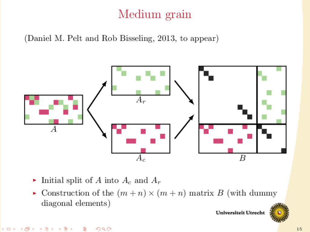
vertices, rows and columns are hyperedges. The nonzero aij is placed in the hyperedges i and j A lot of freedom in partitioning (each nonzero can be assigned individually), but the size of the hypergraph (N vertices) is often too large. medium grain: middle ground between 1-dimensional models and fine-grain Good compromise between the size of the hypergraph and freedom during the partitioning.
of A Development of a fully iterative scheme: lowering the communication value by using information on the previous partitioning These directions can be combined: we can try to find efficient ways of splitting A into Ar and Ac , distinguishing between: partition-oblivious heuristics: no prior information is required partition-aware heuristics: requirement of A already partitioned
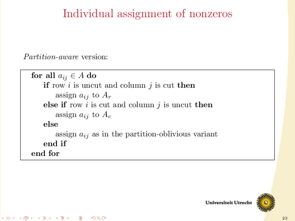
in the construction of the heuristics: short rows/columns (w.r.t. the number of nonzeros) are more likely to be uncut in a good partitioning if a row/column is uncut, the partitioner decided at the previous iteration that it was convenient to do so. We shall try to keep, as much as possible, those rows/columns uncut again.
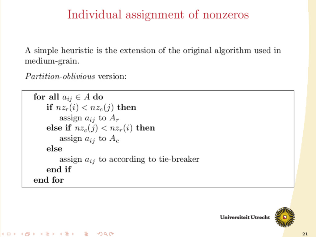
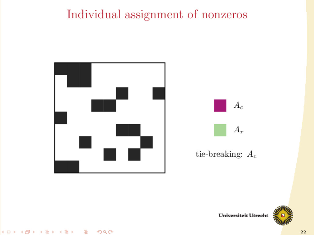
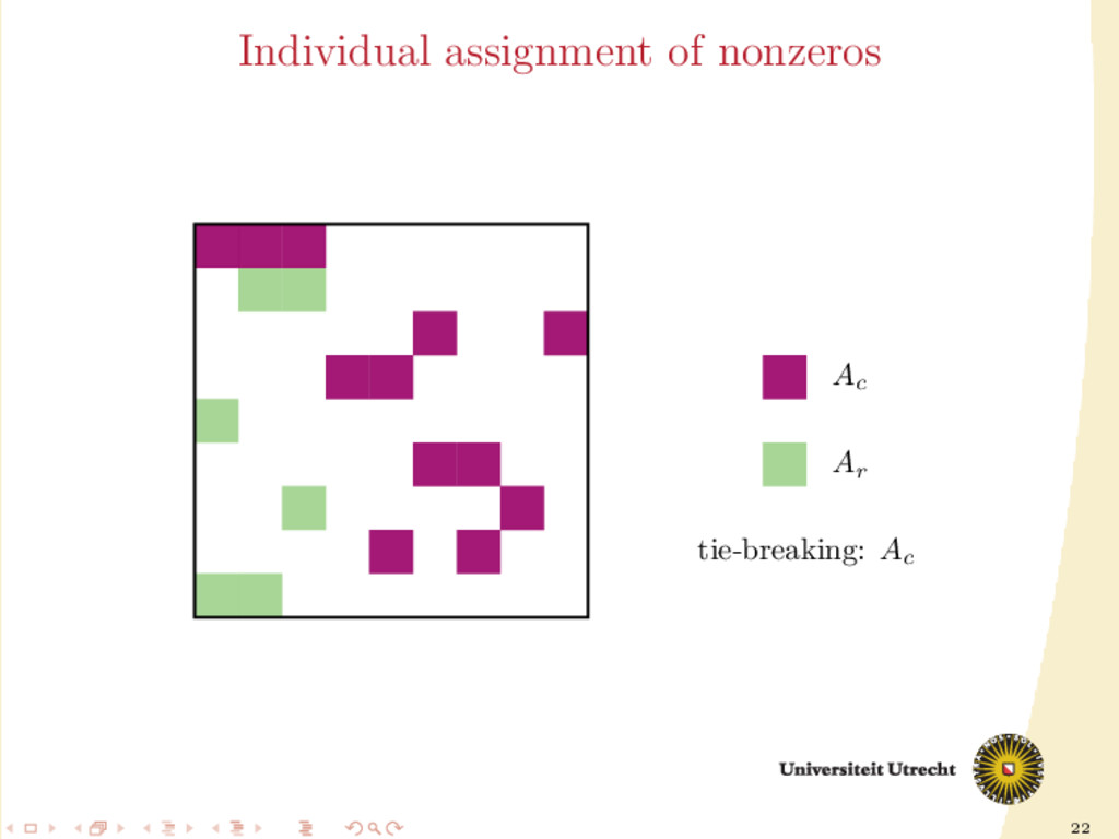
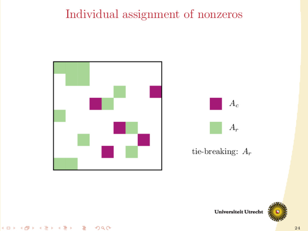
extension of the original algorithm used in medium-grain. Partition-oblivious version: for all aij ∈ A do if nzr (i) < nzc (j) then assign aij to Ar else if nzc (j) < nzr (i) then assign aij to Ac else assign aij to according to tie-breaker end if end for
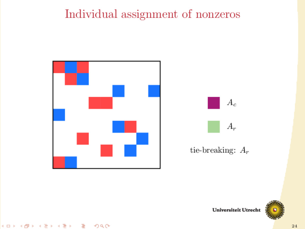
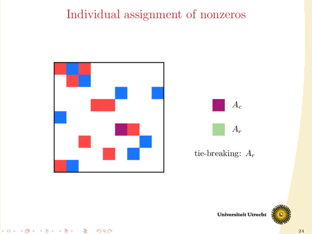
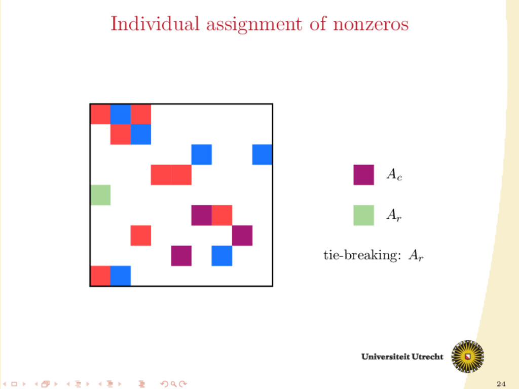
∈ A do if row i is uncut and column j is cut then assign aij to Ar else if row i is cut and column j is uncut then assign aij to Ac else assign aij as in the partition-oblivious variant end if end for
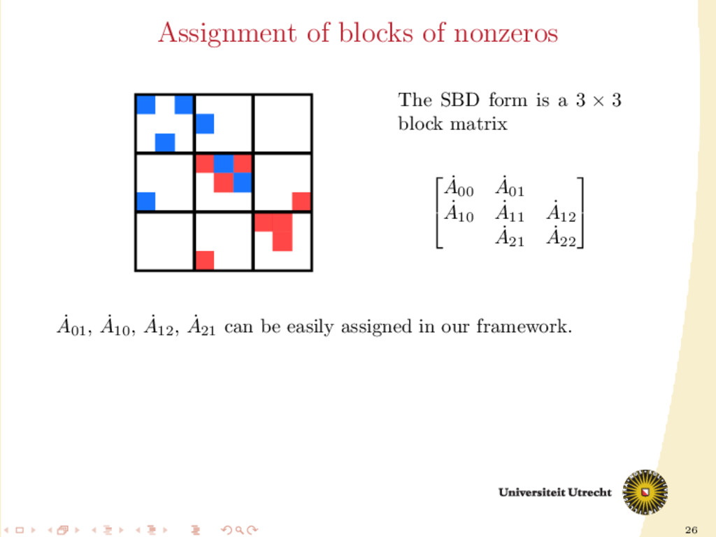
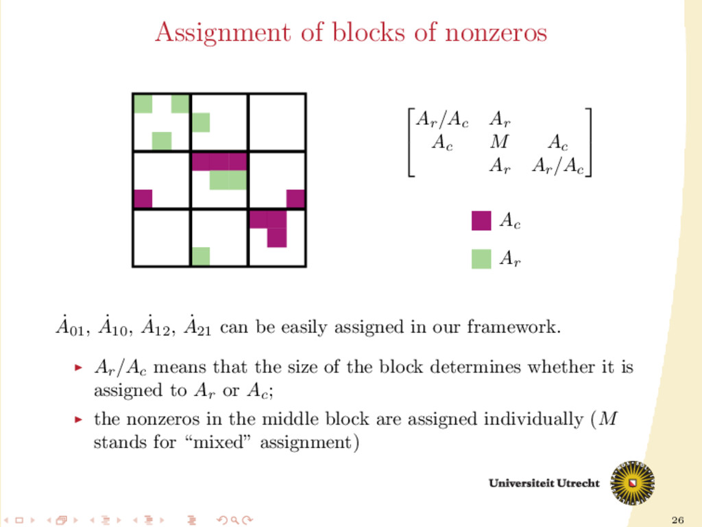
Ar Ac M Ac Ar Ar /Ac Ac Ar ˙ A01 , ˙ A10 , ˙ A12 , ˙ A21 can be easily assigned in our framework. Ar /Ac means that the size of the block determines whether it is assigned to Ar or Ac ; the nonzeros in the middle block are assigned individually (M stands for “mixed” assignment)
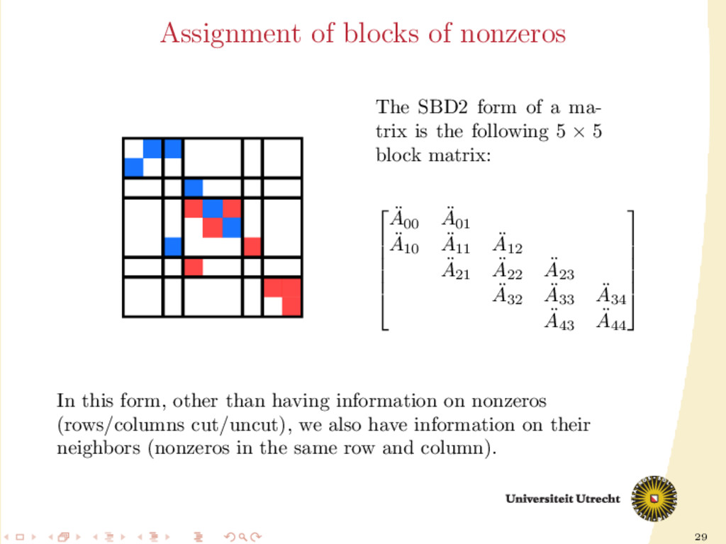
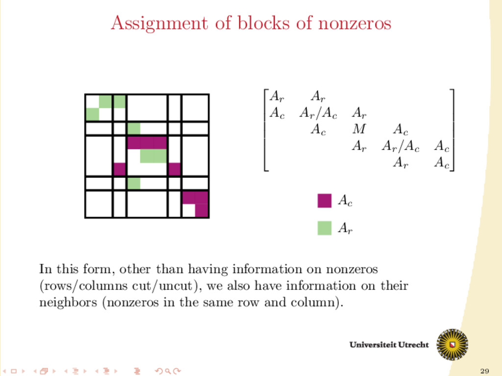
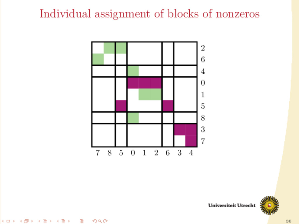
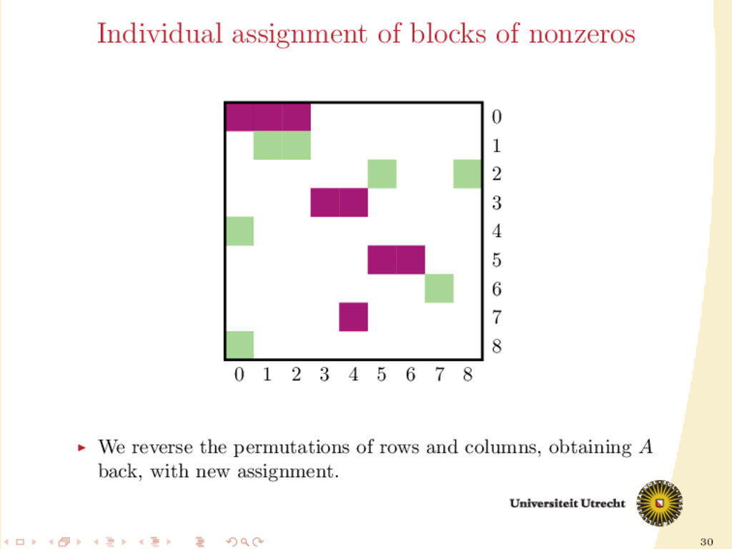
a ma- trix is the following 5 × 5 block matrix: ¨ A00 ¨ A01 ¨ A10 ¨ A11 ¨ A12 ¨ A21 ¨ A22 ¨ A23 ¨ A32 ¨ A33 ¨ A34 ¨ A43 ¨ A44 In this form, other than having information on nonzeros (rows/columns cut/uncut), we also have information on their neighbors (nonzeros in the same row and column).
Ar Ar Ac Ar /Ac Ar Ac M Ac Ar Ar /Ac Ac Ar Ac Ac Ar In this form, other than having information on nonzeros (rows/columns cut/uncut), we also have information on their neighbors (nonzeros in the same row and column).
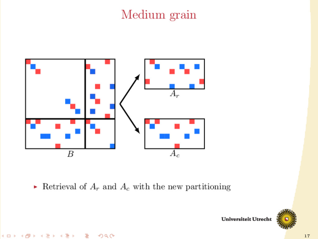
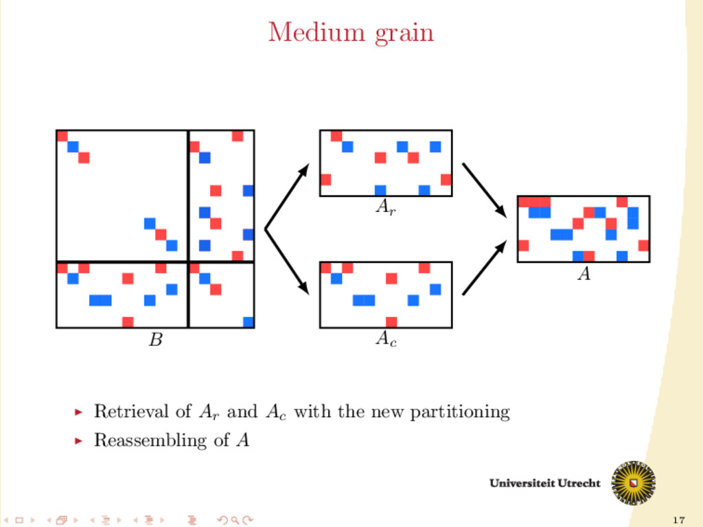
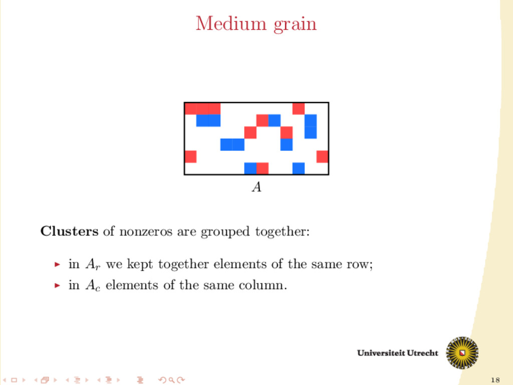
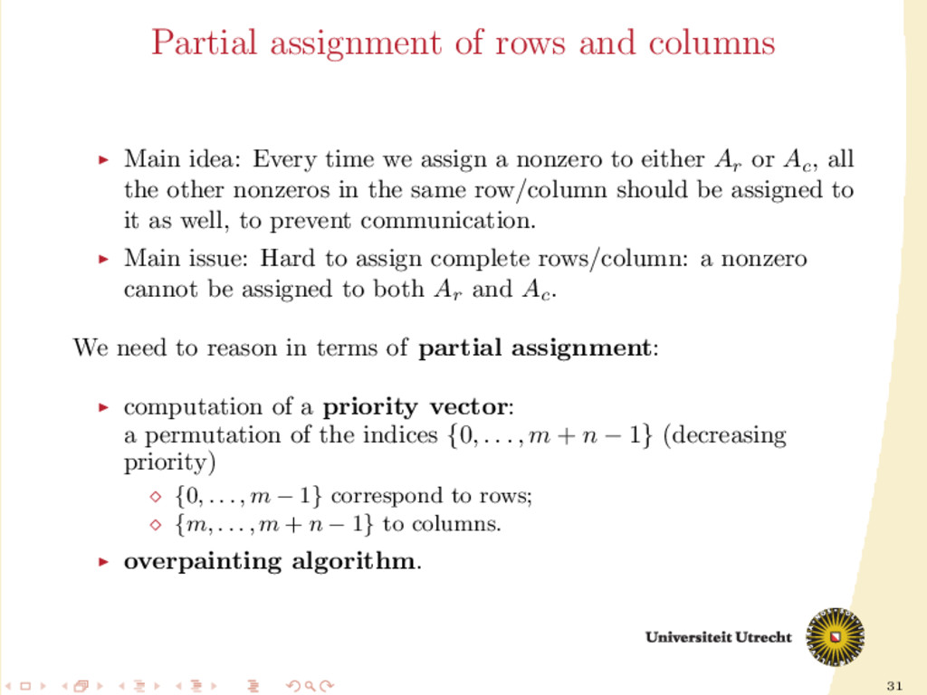
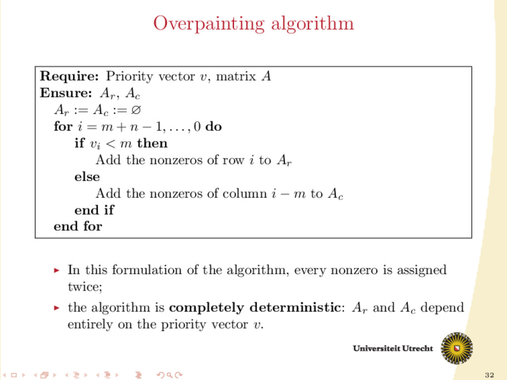
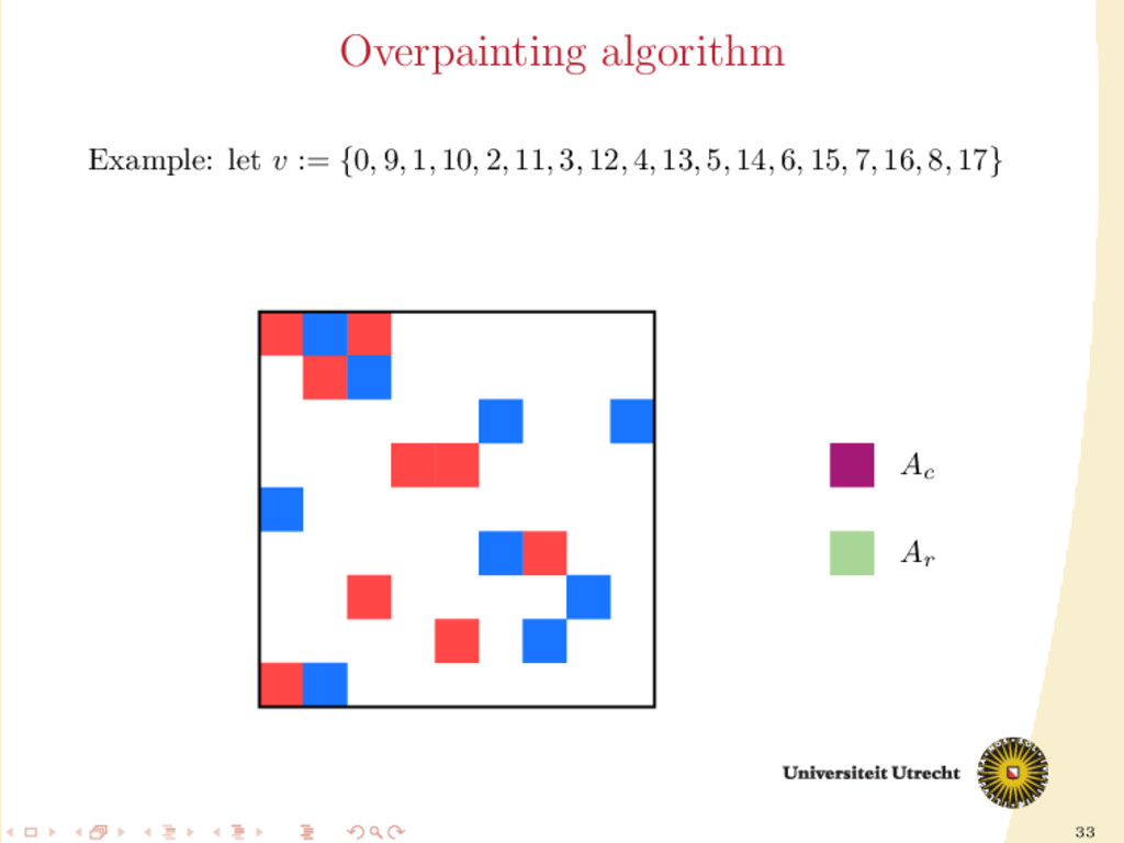
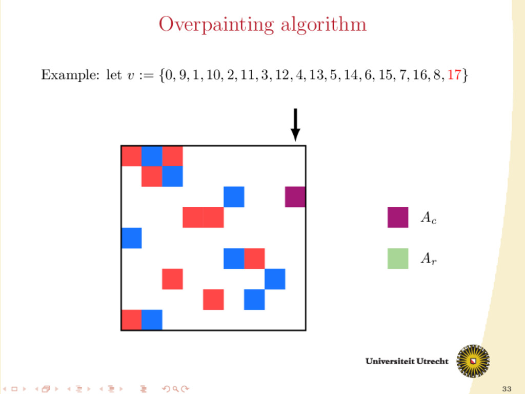
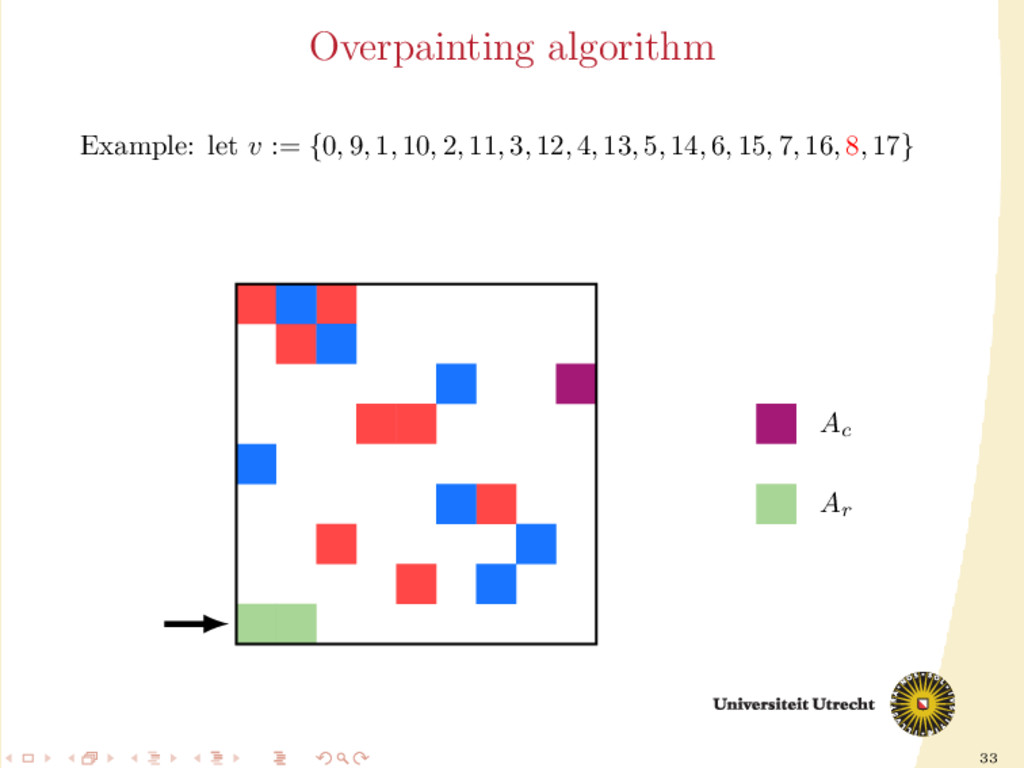
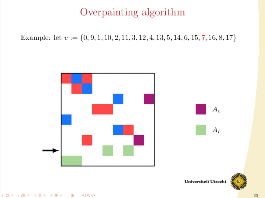
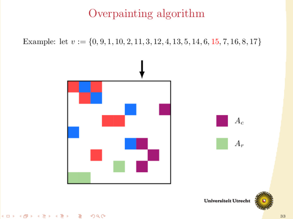
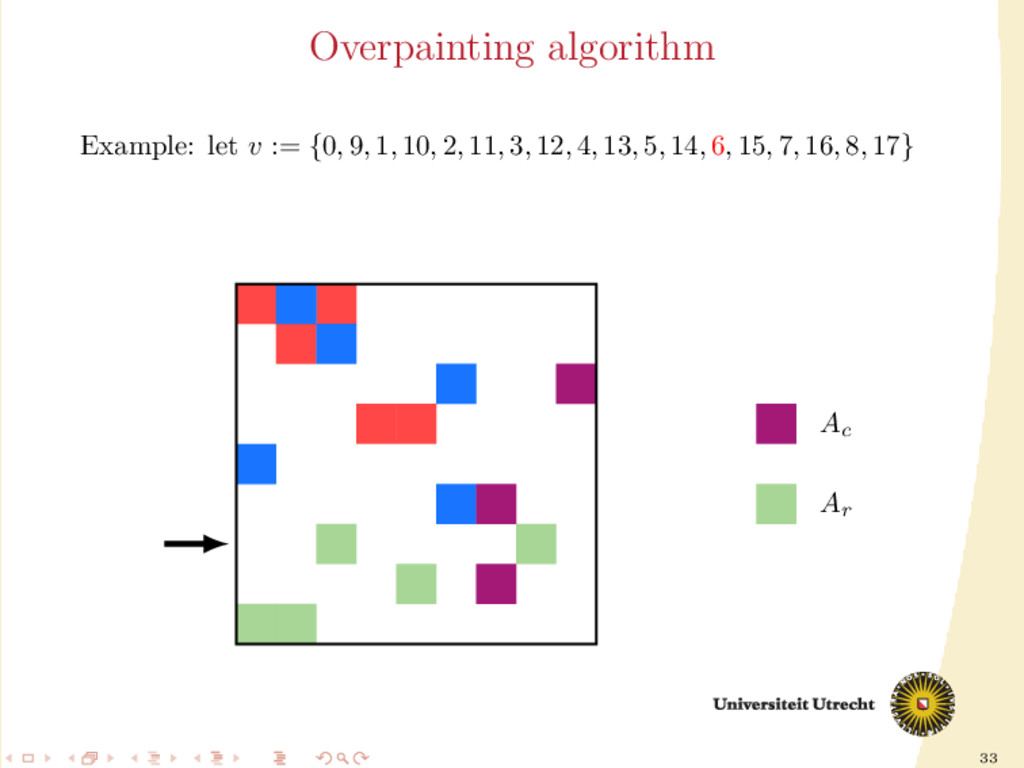
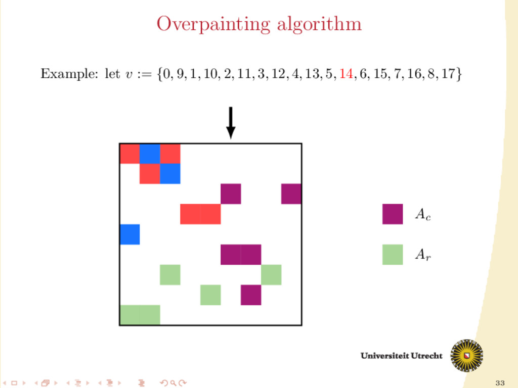
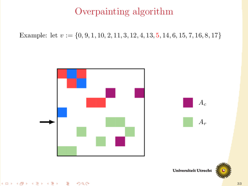
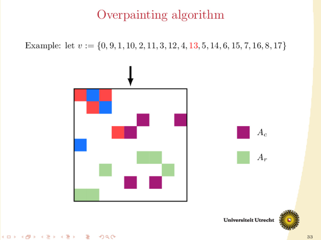
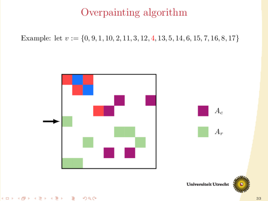
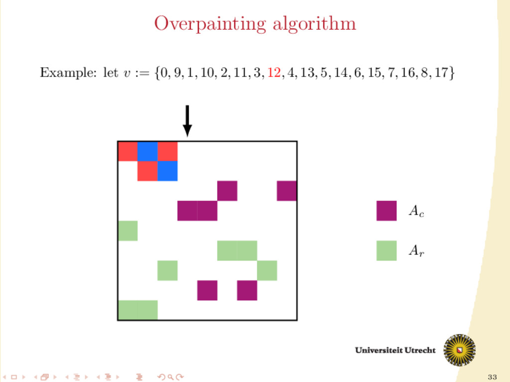
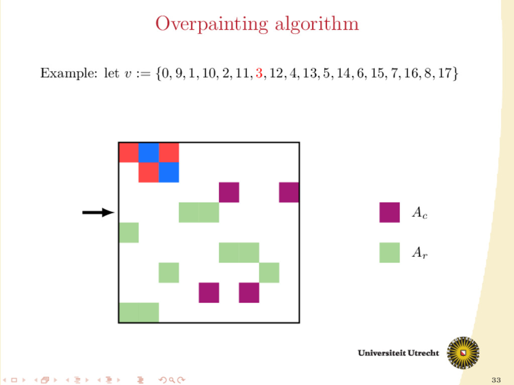
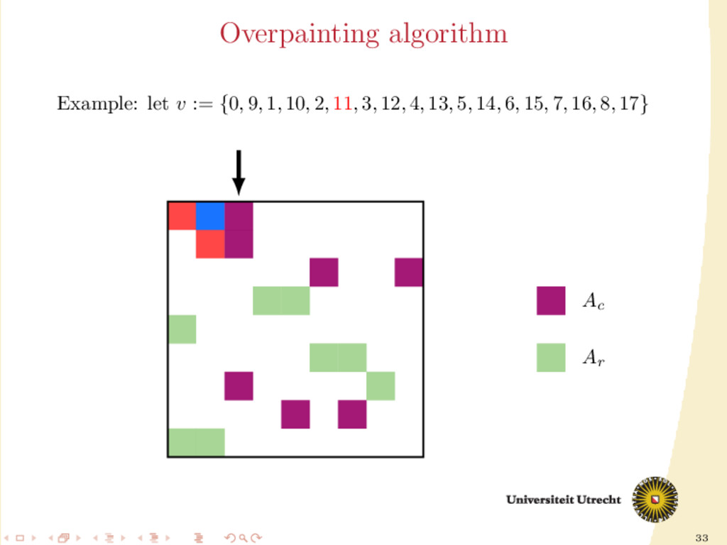
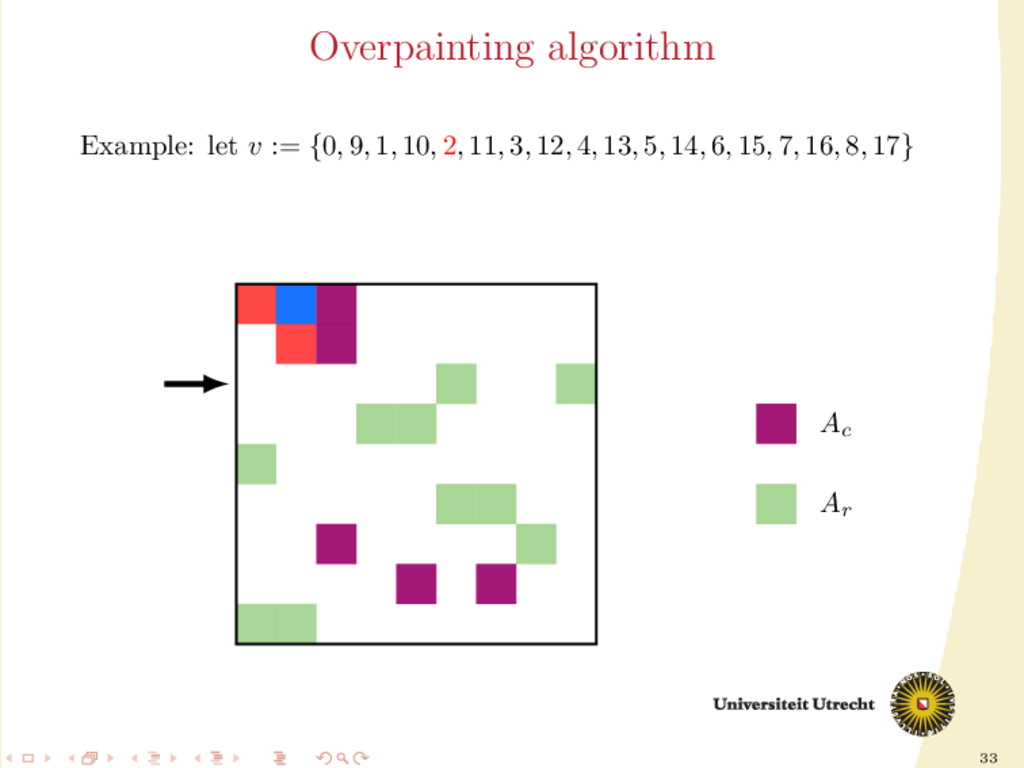
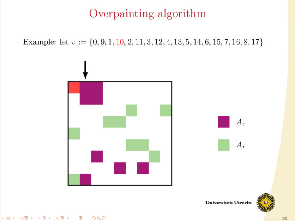
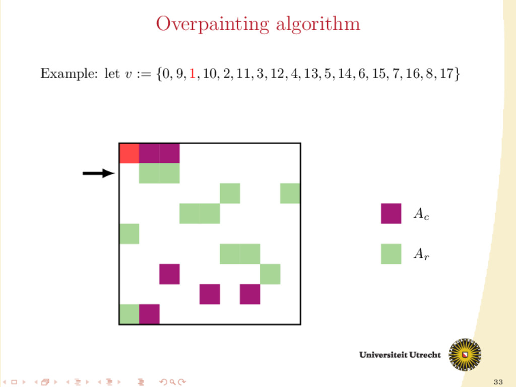
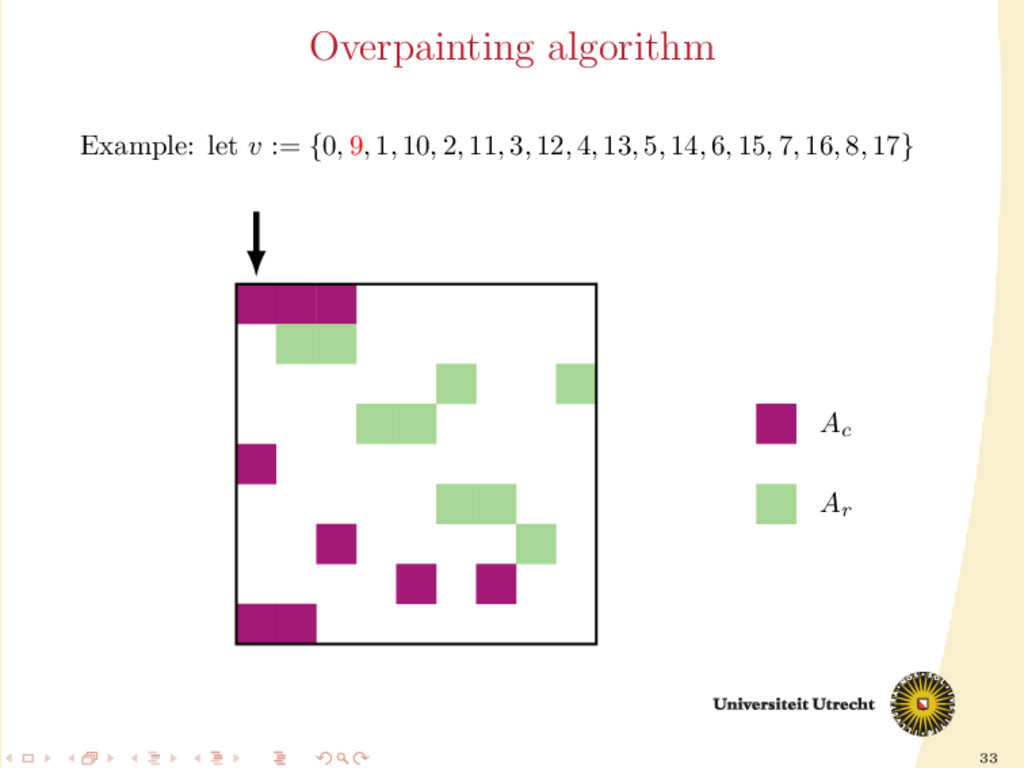
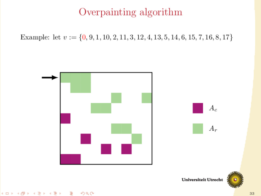
time we assign a nonzero to either Ar or Ac , all the other nonzeros in the same row/column should be assigned to it as well, to prevent communication. Main issue: Hard to assign complete rows/column: a nonzero cannot be assigned to both Ar and Ac . We need to reason in terms of partial assignment: computation of a priority vector: a permutation of the indices {0, . . . , m + n − 1} (decreasing priority) {0, . . . , m − 1} correspond to rows; {m, . . . , m + n − 1} to columns. overpainting algorithm.
Ar , Ac Ar := Ac := ∅ for i = m + n − 1, . . . , 0 do if vi < m then Add the nonzeros of row i to Ar else Add the nonzeros of column i − m to Ac end if end for In this formulation of the algorithm, every nonzero is assigned twice; the algorithm is completely deterministic: Ar and Ac depend entirely on the priority vector v.
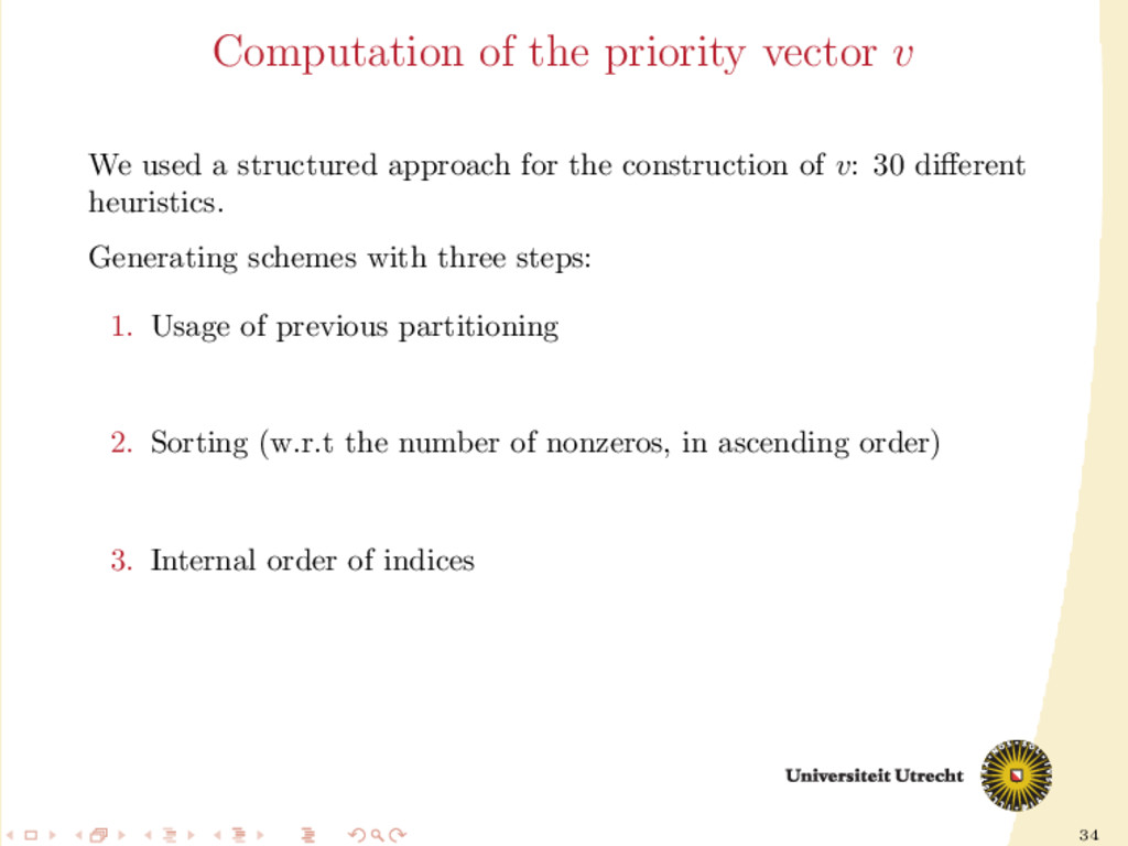
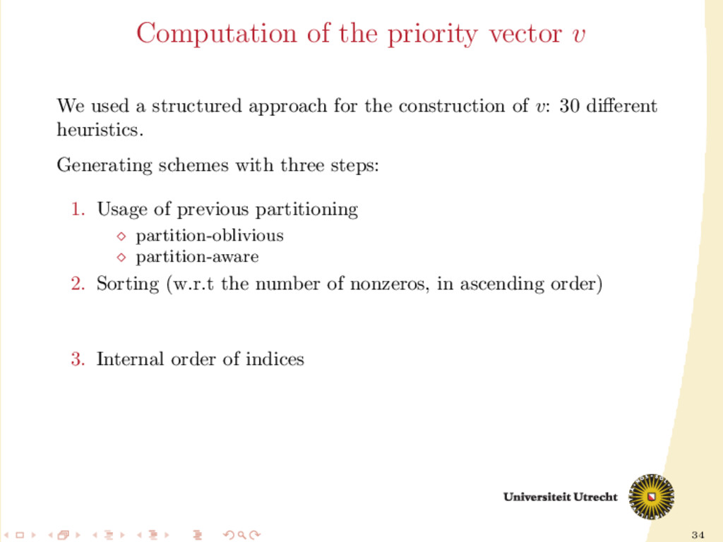
structured approach for the construction of v: 30 different heuristics. Generating schemes with three steps: 1. Usage of previous partitioning 2. Sorting (w.r.t the number of nonzeros, in ascending order) 3. Internal order of indices
structured approach for the construction of v: 30 different heuristics. Generating schemes with three steps: 1. Usage of previous partitioning partition-oblivious partition-aware 2. Sorting (w.r.t the number of nonzeros, in ascending order) 3. Internal order of indices
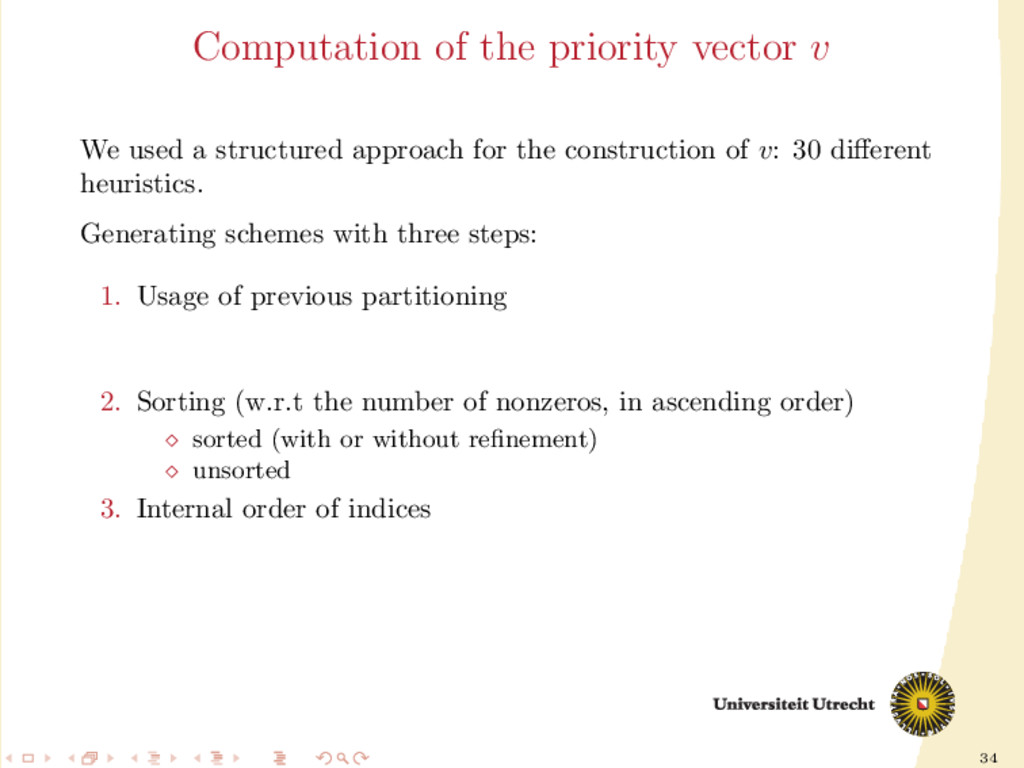
structured approach for the construction of v: 30 different heuristics. Generating schemes with three steps: 1. Usage of previous partitioning 2. Sorting (w.r.t the number of nonzeros, in ascending order) sorted (with or without refinement) unsorted 3. Internal order of indices
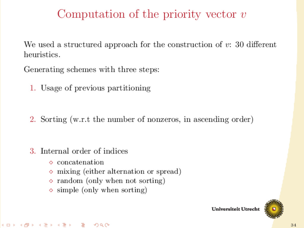
structured approach for the construction of v: 30 different heuristics. Generating schemes with three steps: 1. Usage of previous partitioning 2. Sorting (w.r.t the number of nonzeros, in ascending order) 3. Internal order of indices concatenation mixing (either alternation or spread) random (only when not sorting) simple (only when sorting)
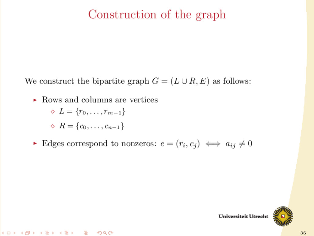
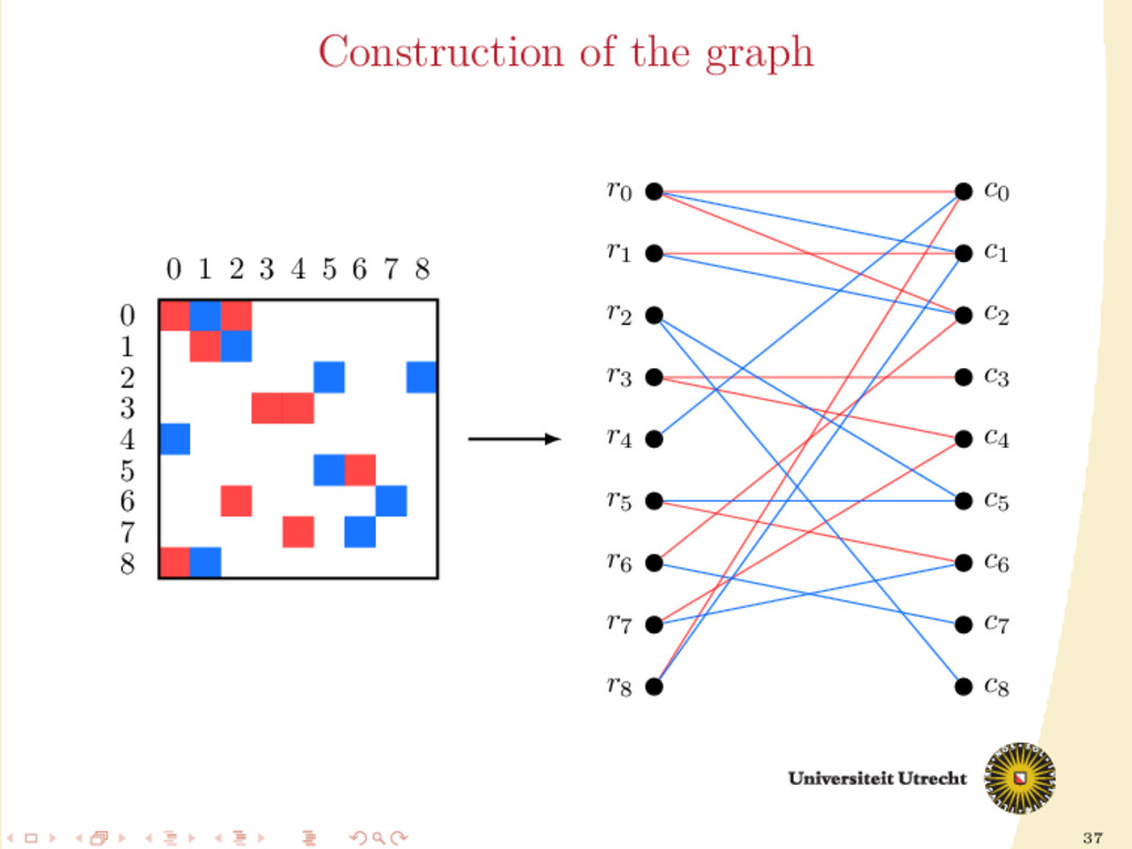
seems an interesting idea, but we want to reduce, as much as possible, the number of cut rows/columns. Goal: Find the biggest subset of {0, . . . , m + n − 1} which can be assigned completely (i.e. full rows and full columns) without causing communication. Graph theory approach: translating the sparsity pattern of A in a particular way, we are looking for a maximum independent set.
subset V ⊆ V such that ∀u, v ∈ V , (u, v) / ∈ E. A maximum independent set is an independent set of G with maximum cardinality. Our desired object is the maximum independent set The complement of a (maximum) independent set is a (minimum) vertex cover
set is as hard as partitioning the matrix (both NP-hard problems). But, luckily, our graph is bipartite: K˝ onig’s Theorem: on bipartite graphs, maximum matchings and minimum vertex covers have the same size; Hopcroft-Karp algorithm: O N √ m + n algorithm to compute a maximum matching on a bipartite graph In our case it is not very demanding to compute a maximum independent set.
let SI denote the maximum independent set computed on the matrix A(I). One partition-oblivious heuristic to compute v: 1. let I = {0, . . . , m + n − 1}, then v := (SI , I \ SI ) For partition-aware heuristics, let U be the set of uncut indices, C be the set of cut indices; we have three possibilities: 1. we compute SU and have v := (SU , U \ SU , C); 2. we compute SU , SC and have v := (SU , U \ SU , SC , C \ SC ); 3. we compute SU , then we define U := U \ SU and compute SC∪U , having v := (SU , SC∪U , (C ∪ U ) \ SC∪U ).
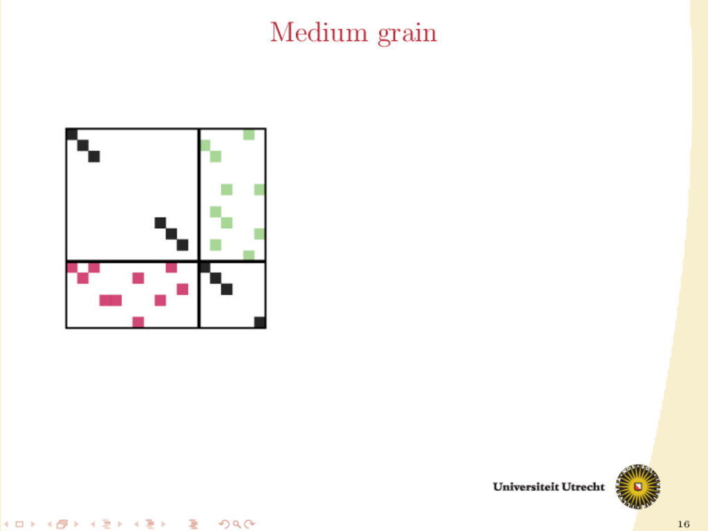
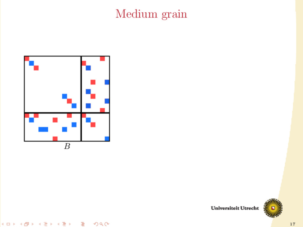
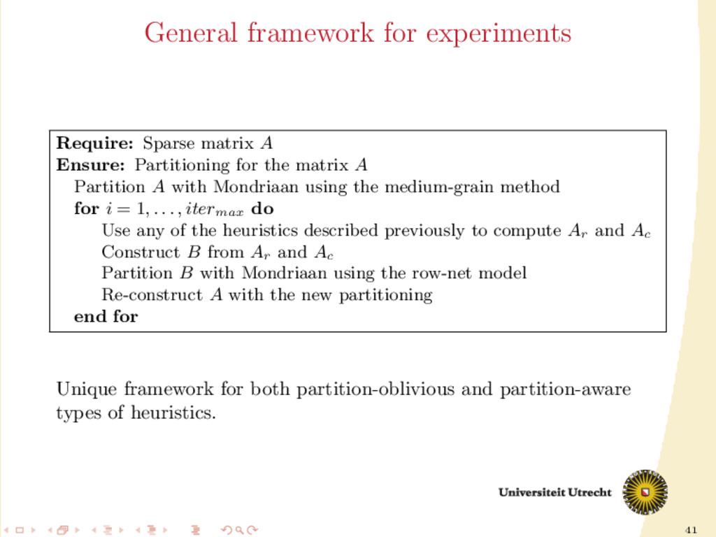
Partitioning for the matrix A Partition A with Mondriaan using the medium-grain method for i = 1, . . . , itermax do Use any of the heuristics described previously to compute Ar and Ac Construct B from Ar and Ac Partition B with Mondriaan using the row-net model Re-construct A with the new partitioning end for Unique framework for both partition-oblivious and partition-aware types of heuristics.
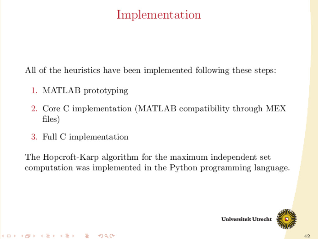
these steps: 1. MATLAB prototyping 2. Core C implementation (MATLAB compatibility through MEX files) 3. Full C implementation The Hopcroft-Karp algorithm for the maximum independent set computation was implemented in the Python programming language.
Ac and during the actual partitioning. To obtain meaningful results: 20 independent initial partitionings for each, 5 independent runs of the heuristic and subsequent partitioning (itermax = 1) 18 matrices used for tests: rectangular vs. square 10th Dimacs Implementation Challenge
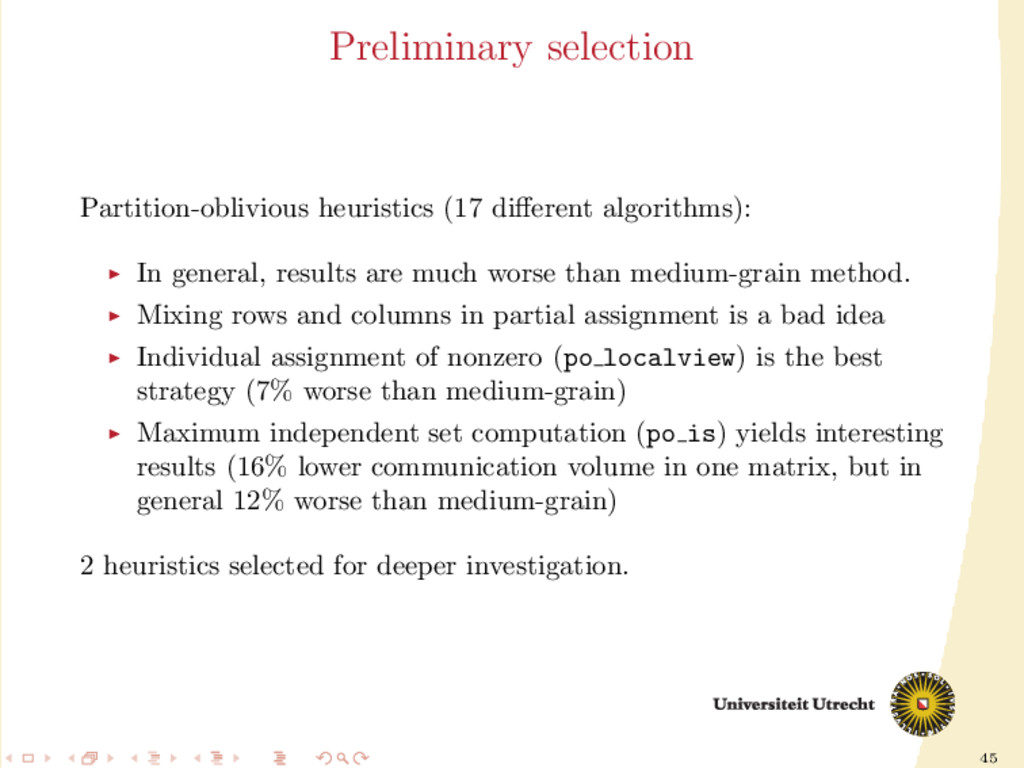
results are much worse than medium-grain method. Mixing rows and columns in partial assignment is a bad idea Individual assignment of nonzero (po localview) is the best strategy (7% worse than medium-grain) Maximum independent set computation (po is) yields interesting results (16% lower communication volume in one matrix, but in general 12% worse than medium-grain) 2 heuristics selected for deeper investigation.
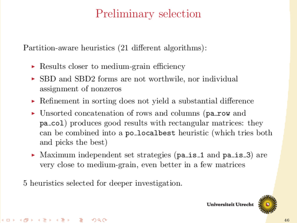
to medium-grain efficiency SBD and SBD2 forms are not worthwile, nor individual assignment of nonzeros Refinement in sorting does not yield a substantial difference Unsorted concatenation of rows and columns (pa row and pa col) produces good results with rectangular matrices: they can be combined into a po localbest heuristic (which tries both and picks the best) Maximum independent set strategies (pa is 1 and pa is 3) are very close to medium-grain, even better in a few matrices 5 heuristics selected for deeper investigation.
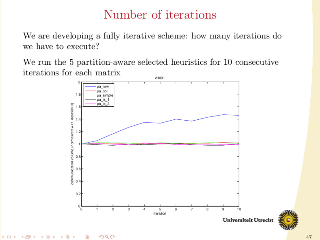
6 7 8 9 10 0 0.2 0.4 0.6 0.8 1 1.2 1.4 1.6 1.8 2 iteration communication volume (normalized w.r.t. iteration 0) dfl001 pa_row pa_col pa_simple pa_is_1 pa_is_3 We are developing a fully iterative scheme: how many iterations do we have to execute? We run the 5 partition-aware selected heuristics for 10 consecutive iterations for each matrix
6 7 8 9 10 0 0.2 0.4 0.6 0.8 1 1.2 1.4 1.6 1.8 2 iteration communication volume (normalized w.r.t. iteration 0) nug30 pa_row pa_col pa_simple pa_is_1 pa_is_3 We are developing a fully iterative scheme: how many iterations do we have to execute? We run the 5 partition-aware selected heuristics for 10 consecutive iterations for each matrix
6 7 8 9 10 0 0.2 0.4 0.6 0.8 1 1.2 1.4 1.6 1.8 2 iteration communication volume (normalized w.r.t. iteration 0) bcsstk30 pa_row pa_col pa_simple pa_is_1 pa_is_3 We are developing a fully iterative scheme: how many iterations do we have to execute? We run the 5 partition-aware selected heuristics for 10 consecutive iterations for each matrix
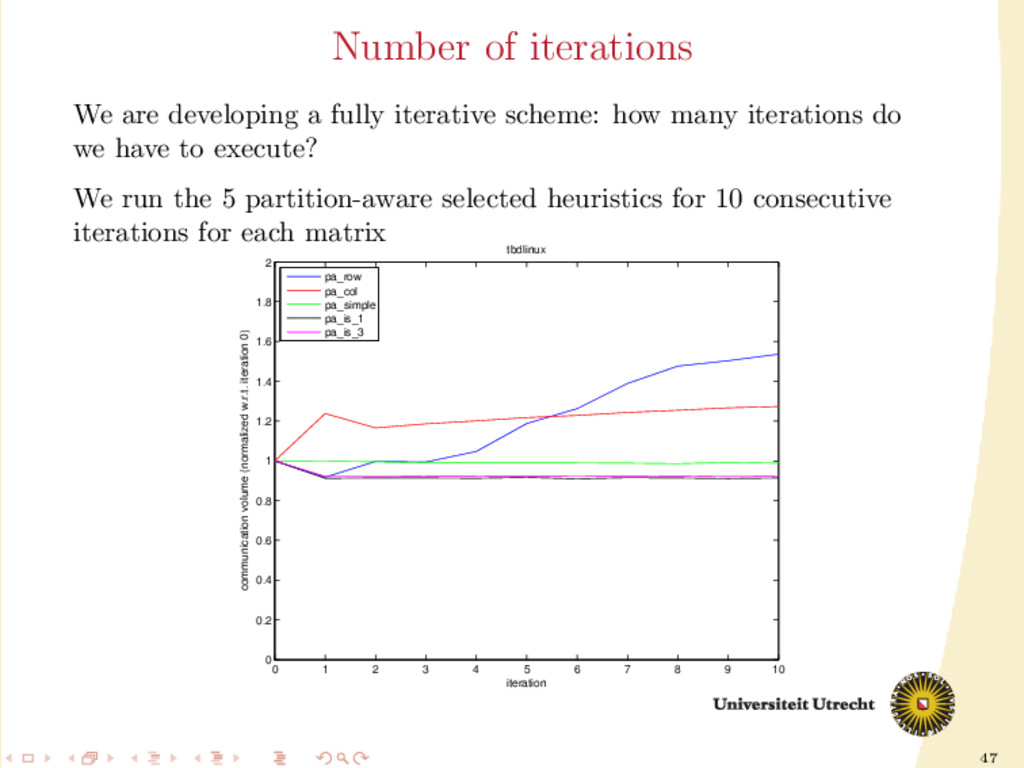
6 7 8 9 10 0 0.2 0.4 0.6 0.8 1 1.2 1.4 1.6 1.8 2 iteration communication volume (normalized w.r.t. iteration 0) tbdlinux pa_row pa_col pa_simple pa_is_1 pa_is_3 We are developing a fully iterative scheme: how many iterations do we have to execute? We run the 5 partition-aware selected heuristics for 10 consecutive iterations for each matrix
6 7 8 9 10 0 0.2 0.4 0.6 0.8 1 1.2 1.4 1.6 1.8 2 iteration communication volume (normalized w.r.t. iteration 0) delaunay_n15 pa_row pa_col pa_simple pa_is_1 pa_is_3 We are developing a fully iterative scheme: how many iterations do we have to execute? We run the 5 partition-aware selected heuristics for 10 consecutive iterations for each matrix
show improvements, if any. More iterations can worsen the communication volume. We are developing a fully iterative scheme: how many iterations do we have to execute? We run the 5 partition-aware selected heuristics for 10 consecutive iterations for each matrix
heuristics: No devised heuristic was able to improve medium-grain The preliminary results confirmed: Individual assignment of nonzeros 7% worse than medium-grain Computing the maximum independent set 22% worse than medium-grain
heuristics: Concatenation interesting strategy: pa row and pa col 8% worse than medium-grain localbest method takes best of both: only 4% worse than medium-grain Similar good results for the other strategies (between 4% and 8% higher communication volume than medium-grain) No algorithm was able to beat medium-grain Considering only rectangular matrices, our methods work better: they improve medium-grain, even if only by little (1-2%)
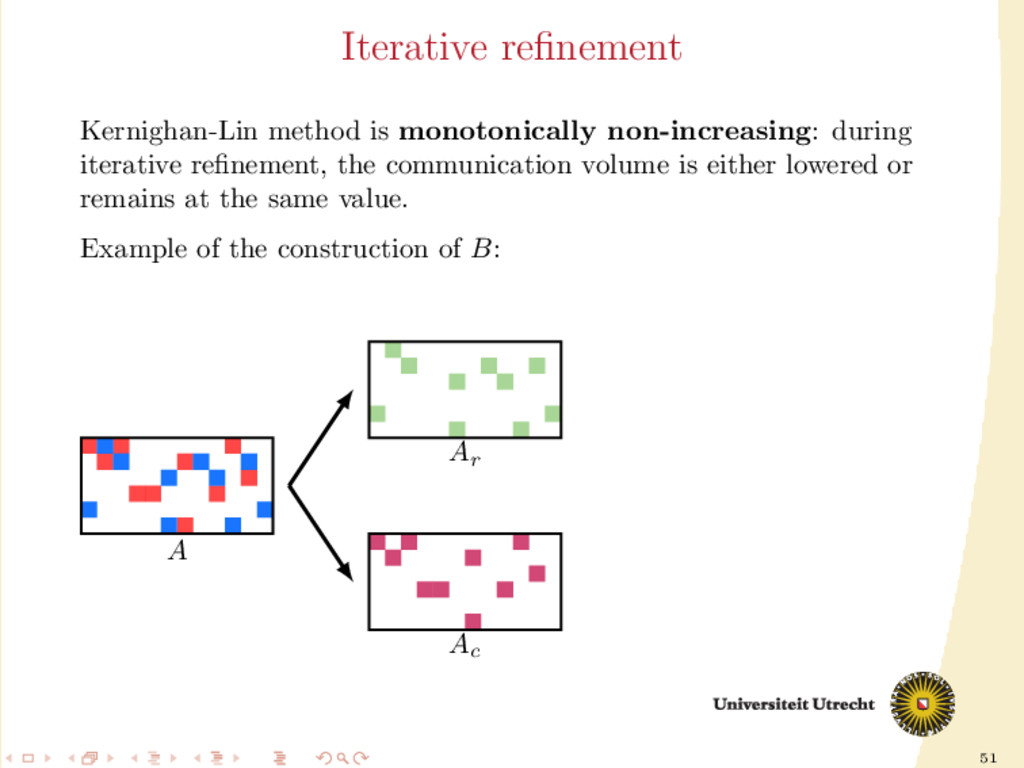
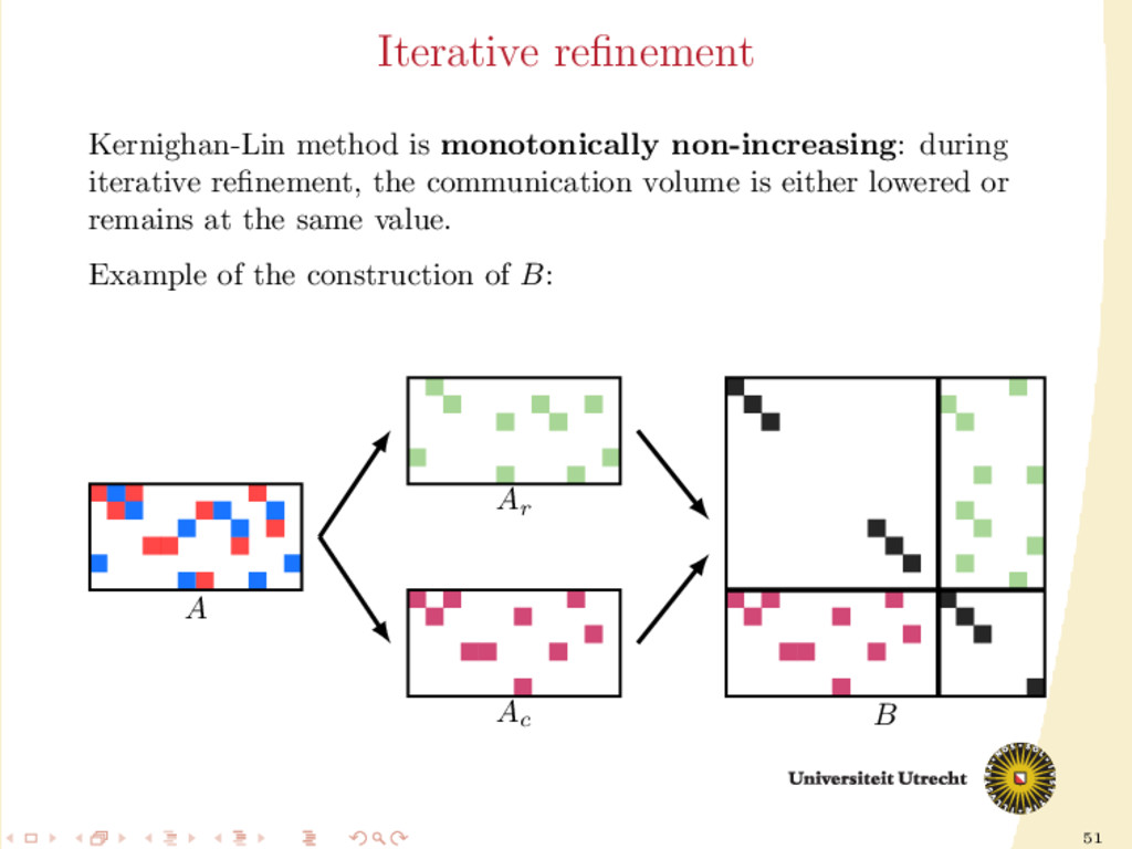
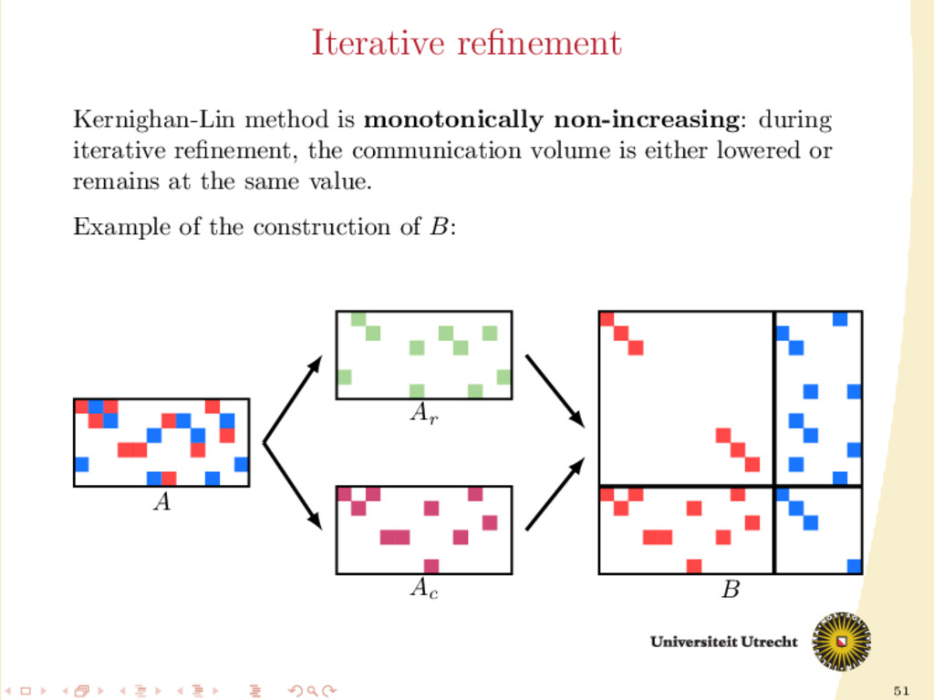
improve the results? Medium-grain employs a procedure of iterative refinement: 1. A is partitioned into two sets (A0 and A1 ) 2. we create again the matrix B of the medium-grain method (example: Ar = A0 and Ac = A1 ) 3. we retain communication volume: the first n columns of B are assigned to a single processor, and similarly for the other m 4. we create the hypergraph from this B and a single run of Kernighan-Lin is performed 5. we repeat steps 1-4 until no improvement is found, then we swap the roles of A0 and A1 for the creation of Ar and Ac 6. we repeat step 5 until no other improvement is found
better: partition-oblivious algorithms: po localview still 7% worse than medium-grain po is now 6% worse than medium-grain (down from 22%) partition-aware algorithms: pa row and pa col now 2% and 1% worse than medium-grain (down from 8%) localbest now 1% better than medium-grain (down from 4% worse) pa simple now 2% worse than medium-grain (down from 4%) pa is 1 and pa is 3 now 1% worse than medium-grain (down from 5% and 8%) Now, with rectangular matrices, computing the independent set produces an average communication volume 4% lower than medium-grain.
quality of the initial partitioning Developing a fully-iterative scheme We were able to outperform medium-grain only by a small margin Computing the independent set is worthwile. Also results about concatenation of rows and columns can be explained with it. Our approach works well with rectangular matrices
Keep testing other strategies to gain more confidence on medium-grain Maximum weighted independent set to maximize the number of nonzeros completely assigned If our approach is confirmed to work consistently well with rectangular matrices, it could be added to Mondriaan: 1. the program detects that the matrix is strongly rectangular and asks user for input; 2. the user decides whether he wants to sacrifice computation time for a better partitioning and execute our approach