EuroPython 2016 - Python, Data & Rock'n'Roll

Have you ever wonder how David Bowie has evolved into the theme of his songs throughout their studio albums? Want to find out in what looks like Nirvana and Pink Floyd?

Approach to topics, evolution, correlations through the lyrics of some of the greatests rock bands of all times. We will talk about the different phases of this personal project, in which I approach to a passion through a scientific method.

This is a project that combine different techniques: - Web crawling - NoSQL - Natural Language Processing - Data visualization

Transcript

1. PYTHON, DATA AND ROCK 'N' ROLL PYTHON, DATA AND ROCK 'N' ROLL EuroPython 2016 EuroPython 2016 Sub Community: PyData Sub Community: PyData Friday 22 July Friday 22 July
2. Who am I? Who am I? Claudia Guirao Fernández Claudia Guirao Fernández @claudiaguirao @claudiaguirao Data Scien�st @ Kernel Analy�cs Learning enthusiast, pythonic & rocker
3. Python... Data... Rock music Python... Data... Rock music
4. EuroPython 2016 related talks: EuroPython 2016 related talks: SCIENTIST MEETS WEB DEV: HOW PYTHON BECAME THE LANGUAGE OF DATA by GAËL VAROQUAUX NLP Un vector por tu palabra by Mai Gimenez I HATE YOU, NLP... ;) by Katharine Jarmul Data Viz INTERACTIVE DATA KUNG FU WITH SHAOLIN by Guillem Duran OMG, BOKEH IS BETTER THAN EVER! by Fablio Pliger Music Talks IMPLEMENTING A SOUND IDENTIFIER IN PYTHON by Cameron Macleod MUSIC TRANSCRIPTION WITH PYTHON by Anna Wszeborowska
5. Development stages Development stages Data grabbing and storage 1. Data processing & term frequency 2. Clustering and topic Modeling 3. Next steps? 4.
6. 1. Data grabbing and storage 1. Data grabbing and storage All the project is based on lyrics 1. Live scrapping soooo much fun :) 2. Web scrapping, fast but less fun All lyrics were scrapped from h�p:/ /www.mldb.org/ I have used requests + beau�ful soup Scrapy, for massive scrapping For convenience data were stored in MongoDB For convenience data were stored in MongoDB from pymongo import MongoClient #mongodb conection client = MongoClient('localhost', 27017) db = client.music collection = db.coolGroups lyrics.append(json)
7. Me doing live scrapping at Pa� Smith concert DISCLAIMER: All groups were selected considering strictly my personal preferences LEGAL DISCLAIMER: All lyrics were scraped from www.mldb.org for my personal learning and entertaiment. Lyrics are intellectual property please manage with care
8. In [1]: from pymongo import MongoClient client = MongoClient('localhost', 27017) db = client.music collection = db.coolGroups cursor = collection.find({"group":"Queen","song": "Don't Stop Me Now "}).limit(1) for doc in cursor: print "group: " + doc["group"] print "album: " + doc["album"] print "song: " + doc["song"] print "url: " + doc["url_scrap"] print "lyrics: " + doc["lyrics"] group: Queen album: Hot Space song: Don't Stop Me Now url: http://www.mldb.org/song-56960-don-t-stop-me-now.html lyrics: Don't Stop Me Now Written by Freddie Mercury Tonight I'm gonna have myself a real good time I feel alive and the world I'll turn it inside out - yeah And floating around in ecstasy So don't stop me now don't stop me 'Cause I'm having a good time having a good time I'm a shooting star leaping through the sky Like a tiger defying the laws of gravity I'm a racing car passing by like Lady Godiva I'm gonna go go go There's no stopping me I'm burnin' through the sky yeah Two hundred degrees That's why they call me Mister Fahrenheit I'm trav'ling at the speed of light I wanna make a supersonic man out of you Don't stop me now I'm having such a good time I'm having a ball Don't stop me now If you wanna have a good time just give me a call Don't stop me now ('Cause I'm having a good time) Don't stop me now (Yes I'm havin' a good time) I don't want to stop at all Yeah, I'm a rocket ship on my way to Mars On a collision course I am a satellite I'm out of control I am a sex machine ready to reload Like an atom bomb about to Oh oh oh oh oh explode I'm burnin' through the sky yeah Two hundred degrees That's why they call me Mister Fahrenheit I'm trav'ling at the speed of light I wanna make a supersonic woman of you Don't stop me don't stop me Don't stop me hey hey hey Don't stop me don't stop me Ooh ooh ooh, I like it Don't stop me don't stop me Have a good time good time Don't stop me don't stop me ah Oh yeah Alright Oh, I'm burnin' through the sky yeah
10. Number of documents Number of documents Number of documents per group db.coolGroups.count() 7237 db.coolGroups.distinct("group").length 51 db.coolGroups.distinct("album").length 544 db.coolGroups.aggregate([{$group: {_id: $group, total: { $sum: 1} } },{$sort:{t otal:-1}}])
11. In [2]: import pandas as pd from pymongo import MongoClient client = MongoClient('localhost', 27017) db = client.music collection = db.coolGroups pipeline = [ {"$group": { "_id": "$group", "total": { "$sum": 1} } }, {"$sort":{"total":-1}} ] agg_group = list(collection.aggregate(pipeline)) rockTF = pd.DataFrame.from_records(agg_group, columns=['total', '_id']) rockTF.sort_values('total', ascending=False).head(10) Out[2]: total _id 0 431 Bruce Springsteen 1 429 Aerosmith 2 381 Pink Floyd 3 339 Bob Dylan 4 332 Queen 5 309 The Beatles 6 266 David Bowie 7 263 The Clash 8 255 T-Rex 9 244 R.E.M.
12. In [3]: %matplotlib inline from os import path from PIL import Image import numpy as np import matplotlib.pyplot as plt from wordcloud import WordCloud client = MongoClient('localhost', 27017) db = client.music collection = db.coolGroups cursor = collection.find({},{ "group": 1, "_id": 0 } ) corpus="" for doc in cursor: corpus = corpus + " " + doc["group"] snake_mask = np.array(Image.open("python snake.png")) wc = WordCloud(background_color="white", max_words=100, mask=snake_mask) wc.generate(corpus) Out[3]: <wordcloud.wordcloud.WordCloud at 0x7fbf34097fd0>
13. In [4]: plt.imshow(wc) plt.axis("off") plt.figure() plt.imshow(snake_mask, cmap=plt.cm.gray) plt.axis("off") plt.show()
14. 2. Data processing 2. Data processing Stopwords 1. Words Tokens Lemmas 2. Rock Index 3. Term Frequencies and another curiosi�es 4.
15. NLP can be defined as the automa�c or semi-automa�c processing of human language. NLP is essen�ally mul�disciplinary: closely related to linguis�cs, it also has links to research in cogni�ve science, psychology, philosophy and maths (especially logic) It is also related with machine learning. We have to clean our lyrics from meaningless words, puntua�on, etc. In [5]: from collections import Counter import nltk from nltk import word_tokenize from nltk.corpus import stopwords, brown from nltk.stem.snowball import SnowballStemmer import string import re
16. Also there are a bunch of meaningless words that we would want to avoid, they are called stopwords. In the music field also. In [6]: # load nltk's English stopwords as variable called 'stopwords' stopwords = nltk.corpus.stopwords.words('english') stopwords_music = ["chorus", "x2","x3","x4","ohh" "ooh","oooh","uh","uuh","uuuh", "ya","la","da","na","ha", "ah","aah","ahh","yeah","oh","instrume ntal", "ha","re", "a","repeat"] stopwords_full = stopwords + stopwords_music
17. In [7]: import re cList = { "ain't": "am not", "aren't": "are not", "can't": "cannot", "can't've" : "cannot have", "'cause": "because", "could've": "could have", "couldn't": "could not", "could n't've": "could not have", "didn't": "did not", "doesn't": "does not", "don't": "do not", "hadn't": "had not", "hadn't've": "had not have", "hasn't": "has not", "haven't": "have not", "he'd ": "he would", "he'd've": "he would have", "he'll": "he will", "he'll've": "he will have", "h e's": "he is", "how'd": "how did", "how'd'y": "how do you", "how'll": "how will", "how's": "h ow is", "i'd": "i would", "i'd've": "i would have", "i'll": "i will", "i'll've": "i wi ll have", "i'm": "i am", "i've": "i have", "isn't": "is not", "it'd": "it had", "it'd'v e": "it would have", "it'll": "it will", "it'll've": "it will have", "it's": "it is", "let's": "let us", "ma'am": "madam", "mayn't": "may not", "might've": "might have", "mightn't": "might not", "might n't've": "might not have", "must've": "must have", "mustn't": "must not", "mustn't've": "must not have", "needn't": "need not", "needn't've": "need not have", "o'clock": "of the clock", "oughtn't": "ought no t", "oughtn't've": "ought not have", "shan't": "shall not", "sha'n't": "shall not", "shan't've": "shall not have", "she'd": "she would", "she'd've": "she would have", "she'll": "she will", "she 'll've": "she will have", "she's": "she is", "should've": "should have", "shouldn't": "should not", "sho uldn't've": "should not have", "so've": "so have", "so's": "so is", "that'd": "that would", "that'd've": "tha t would have", "that's": "that is", "there'd": "there had", "there'd've": "there would have", "there's": "there is", "they'd": "they would", "they'd've": "they would have", "they'll": "they will", "they'll've": "they will have", "they're": "they are", "they've": "they have", "to've": "to have", "wasn't": "was not", "we'd": "we had", "we'd've": "we would have", "we'll": "w e will", "we'll've": "we will have", "we're": "we are", "we've": "we have", "weren't": "were not", "what'll": "what will", "what'll've": "what will have", "what're": "what are", "what's": "what is", "what've": "what have", "when's": "when is", "when've": " when have", "where'd": "where did", "where's": "where is", "where've": "where have", "who' ll": "who will", "who'll've": "who will have", "who's": "who is", "who've": "who have", "why's" : "why is", "why've": "why have", "will've": "will have", "won't": "will not", "won't've": "will not have", "would've": "would have", "wouldn't": "would not", "wouldn't've": "would not ha ve", "y'all": "you all", "y'alls": "you alls", "y'all'd": "you all would", "y'all'd 've": "you all would have", "y'all're": "you all are", "y'all've": "you all have", "you'd": "you had", "yo u'd've": "you would have", "you'll": "you you will", "you'll've": "you you will have", "you're": "you are" , "you've": "you have"} c_re = re.compile('(%s)' % '|'.join(cList.keys())) def expandContractions(text, c_re=c_re): def replace(match): return cList[match.group(0)] return c_re.sub(replace, text.lower())
18. In [ ]: # set stemmers porter = nltk.PorterStemmer() lancaster = nltk.LancasterStemmer() snowball = SnowballStemmer("english") wnl = nltk.WordNetLemmatizer() # Mongodb conection client = MongoClient('localhost', 27017) db = client.music collection = db.coolGroups #source collection_dest = db.coolGroupsProcessed #destination cursor = collection.find() for i, document in enumerate(cursor): raw = document["lyrics"].lower() # expand contractions,remove punctuation and stopwords raw = expandContractions(raw) raw = "".join(l for l in raw if l not in string.punctuation) raw = ' '.join([word for word in raw.split() if word not in stopwords_full]) words = re.findall(r'[a-z]+',raw) #tokenize lyrics tokens = word_tokenize(raw) tokens = list((tokens)) # porter stems porter_stems = [porter.stem(t) for t in tokens] porter_stems = list(porter_stems) document["words"]= words document["tokens"]= tokens document["porter_stems"] = porter_stems # save documents in destination collection_dest.insert_one(document)
19. Rockness index Rockness index It is built comparing the TF in our lyrics with the It is built comparing the TF in our lyrics with the brown corpus Note: The Brown Corpus was compiled in the 1960s at Brown University as a general corpus (text collec�on) in the field of corpus linguis�cs. It contains 500 samples of English-language text, totaling roughly one million words, compiled from works published in the United States in 1961. Unfortunately it doesn't take into account lyrics.
20. In [8]: from numpy import log # retrieve all lyrics words client = MongoClient('localhost', 27017) db = client.music collection = db.coolGroupsProcessed cursor = collection.find({},{"tokens":1}) # Rock corpus rock_corpus = [] for i, document in enumerate(cursor): raw = document["tokens"] rock_corpus = rock_corpus + raw rockTF = dict(Counter(rock_corpus)) rockTF = pd.DataFrame(rockTF.items(), columns=['term', 'TF']) rockTF = rockTF.assign(DistrFreq = rockTF.TF/sum(rockTF.TF)) rockTF = rockTF[rockTF['TF'] > 5] #brown corpus brown = brown.words() brownTF = nltk.FreqDist(w.lower() for w in brown) brownTF = dict(brownTF) brownTF = pd.DataFrame(brownTF.items(), columns=['term', 'TFbrown']) brownTF = brownTF[~brownTF.term.isin(stopwords_full)] brownTF = brownTF.assign(DistrFreqbrown = brownTF.TFbrown/sum(brownTF.TFbrown)) brownTF = brownTF[brownTF['TFbrown'] > 5] In [9]: result = pd.merge(rockTF,brownTF, on=['term']) result = result.assign(RocknessIndex = log(result['DistrFreq']/result['DistrFreqbro wn']))
21. In [10]: result.sort_values('RocknessIndex', ascending=False).head(10) #rocking words Out[10]: term TF DistrFreq TFbrown DistrFreqbrown RocknessIndex 265 hey 2077 0.003013 15 0.000022 4.929207 1237 goodbye 480 0.000696 6 0.000009 4.380604 460 babe 517 0.000750 8 0.000012 4.167179 461 baby 3881 0.005629 62 0.000090 4.135291 2990 kiss 563 0.000817 17 0.000025 3.498644 511 tonight 1254 0.001819 38 0.000055 3.495085 2652 love 7573 0.010985 231 0.000336 3.488504 2662 honey 780 0.001131 25 0.000036 3.438996 3805 burn 433 0.000628 15 0.000022 3.361265 2791 hello 283 0.000410 10 0.000015 3.341439
22. In [11]: result.sort_values('RocknessIndex', ascending=True).head(10) #not rocking words Out[11]: term TF DistrFreq TFbrown DistrFreqbrown RocknessIndex 355 also 20 0.000029 1069 0.001553 -3.980169 1612 members 7 0.000010 325 0.000472 -3.839338 1932 however 12 0.000017 552 0.000802 -3.830064 4798 united 11 0.000016 482 0.000700 -3.781471 1529 general 15 0.000022 498 0.000723 -3.503972 2758 schools 6 0.000009 195 0.000283 -3.482663 25 example 9 0.000013 292 0.000424 -3.480952 2492 military 7 0.000010 212 0.000308 -3.412099 4443 several 13 0.000019 377 0.000548 -3.368718 2670 data 6 0.000009 173 0.000251 -3.362955
23. Term Frequencies Term Frequencies In [12]: %matplotlib inline from pymongo import MongoClient client = MongoClient('localhost', 27017) db = client.music collection = db.coolGroupsProcessed cursor = collection.find() rock_corpus = " " rock_text = [] for i, document in enumerate(cursor): raw = document["words"] rock_text = rock_text + raw raw= " ".join(str(x) for x in raw) rock_corpus = rock_corpus + " " + raw rockTF = dict(Counter(rock_text)) rockTF = pd.DataFrame(rockTF.items(), columns=['term', 'TF']) rockTF.sort_values('TF', ascending=False).head(10) Out[12]: term TF 14226 love 7573 8023 know 6818 23715 got 6127 9839 like 6009 7929 get 5019 1178 one 5014 19252 go 4748 14124 �me 4484 15486 see 4179 24771 come 4123
24. In [14]: wc = WordCloud(max_words=300, margin=10,random_state=1).generate(rock_corpus) plt.imshow(wc.recolor(color_func=grey_color_func, random_state=3)) plt.axis("off") plt.show()
25. In [16]: TFworcloud("Queen") Queen term TF 919 love 1090 249 one 917 946 ooh 674 1667 go 520 1521 hey 454
26. In [17]: TFworcloud("The Beatles") The Beatles term TF 712 love 765 2232 know 580 922 say 295 972 get 292 1859 let 285
27. In [18]: TFworcloud("David Bowie") David Bowie term TF 2311 like 264 711 love 227 2626 got 177 3565 time 176 1102 know 156
28. In [19]: TFworcloud("nirvana") nirvana term TF 918 way 107 1802 know 95 132 would 88 1814 like 88 1469 take 80
29. Have rock lyrics an extensive vocabulary? Have rock lyrics an extensive vocabulary? In [20]: client = MongoClient('localhost', 27017) db = client.music collection = db.coolGroupsProcessed pipeline= [ {"$unwind": "$tokens"}, {"$group":{"_id": { "group": "$group"}, "tokens": {"$addToSet": "$tokens" }}}] tokens_bygroup = list(collection.aggregate(pipeline)) groupedby = [] for agg in tokens_bygroup: vocab={} group = agg["_id"] group = group["group"] countdistinct = len(agg["tokens"]) vocab["group"] = group vocab["count"] = countdistinct groupedby.append(vocab) vocabDF = pd.DataFrame.from_records(groupedby, columns=['group', 'count'])
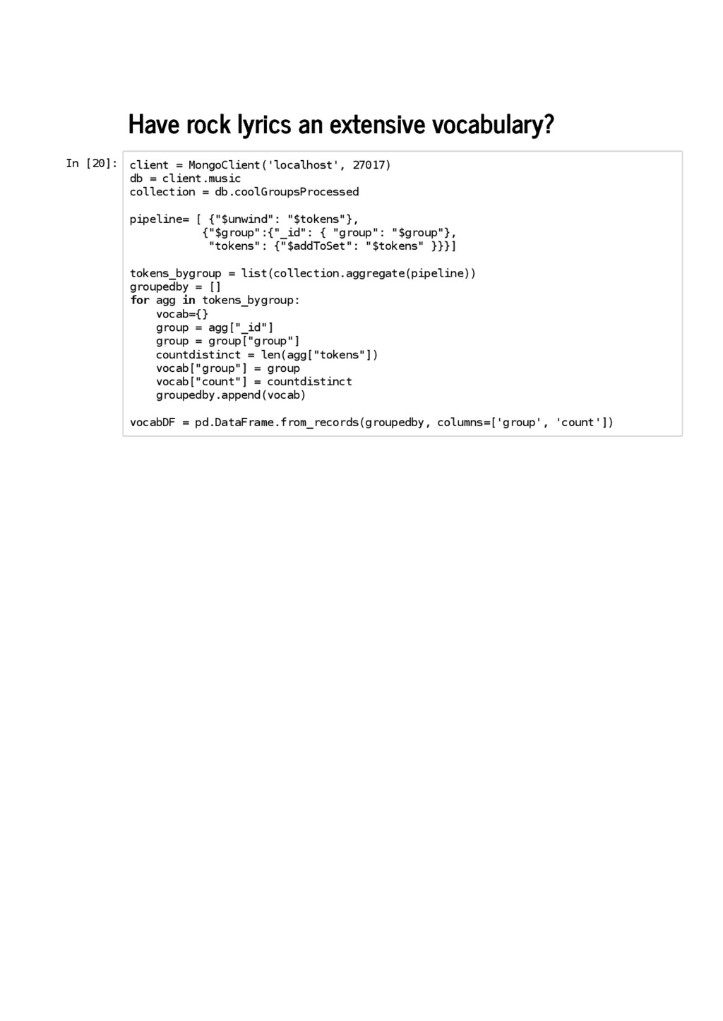
30. In [21]: vocabDF.sort_values('count', ascending=False).head() Out[21]: group count 39 Bob Dylan 7089 30 Bruce Springsteen 5781 44 David Bowie 4820 2 R.E.M. 4429 23 Red Hot Chili Peppers 4190
31. In [22]: vocabDF.sort_values('count', ascending=True).head() Out[22]: group count 37 AC/DC 498 49 Kasabian 509 9 Motorhead 559 6 A Perfect Circle 823 7 Jane's Addic�on 854
32. In [23]: client = MongoClient('localhost', 27017) db = client.music collection = db.coolGroupsProcessed pipeline= [ {"$unwind": "$tokens"}, {"$group":{"_id": { "group": "$group", "song":"$song"}, "tokens": {"$addToSet": "$tokens" }}}] tokens_bygroup = list(collection.aggregate(pipeline)) groupedby = [] for agg in tokens_bygroup: vocab={} ids = agg["_id"] group = ids["group"] song = ids["song"] countdistinct = len(agg["tokens"]) vocab["group"] = group vocab["count"] = countdistinct vocab["song"] = song groupedby.append(vocab) vocabDF = pd.DataFrame.from_records(groupedby, columns=['group','song','count']) vocabDF.head() vocabDF = vocabDF.groupby(['group']).mean()
33. In [24]: vocabDF.sort_values('count', ascending=False).head() Out[24]: count group Rage Against The Machine 93.943396 Bob Dylan 88.713864 Bruce Springsteen 86.511182 Pa� Smith 78.893939 Pulp 77.974138
34. In [25]: vocabDF.sort_values('count', ascending=True).head() Out[25]: count group Radiohead 32.395522 ramones 35.395480 T-Rex 36.484375 The Beatles 36.577465 nirvana 36.763158
35. Sex? and drugs? and Rock’n’roll Sex? and drugs? and Rock’n’roll In [26]: client = MongoClient('localhost', 27017) db = client.music collection = db.coolGroupsProcessed pipeline = [ {"$unwind": "$tokens"},{"$match":{"tokens": { "$in": ["love","kiss","s ex"] }}}, {"$group":{"_id": { "song": "$song"}, "tokens": {"$addToSet": "$tokens" }}}] lovesongs = list(collection.aggregate(pipeline)) print(len(lovesongs)) 1755
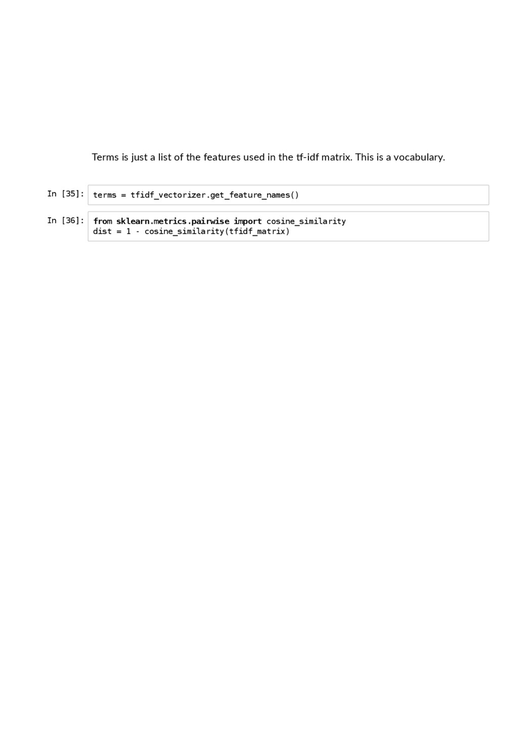
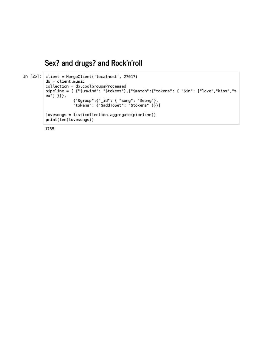
36. In [27]: client = MongoClient('localhost', 27017) db = client.music collection = db.coolGroupsProcessed pipeline = [ {"$unwind": "$tokens"},{"$match":{"tokens": "drug"}}, {"$group":{"_id": { "song": "$song"}, "tokens": {"$addToSet": "$tokens" }}}] drugsongs = list(collection.aggregate(pipeline)) print(len(drugsongs)) 24
38. 3. Clustering and topic modeling 3. Clustering and topic modeling By this point, we already know that: However we are going to try another more sofis�cated techniques * Grouping by band or music groups let us only a few documents (52 groups) * Rock has not a extensive vocabulary * We have the intuition that all the rock songs are talking about the same
39. In [28]: import numpy as np import pandas as pd from sklearn import feature_extraction import mpld3 import os import codecs
40. Define two func�ons: tokenize_and_stem: tokenizes (splits the lyrics into a list of its respec�ve words (or tokens) and also stems each token tokenize_only: tokenizes the synopsis only 1. In [29]: # load nltk's SnowballStemmer as variabled 'stemmer' from nltk.stem.snowball import SnowballStemmer stemmer = SnowballStemmer("english") # here I define a tokenizer and stemmer which returns the set of stems in the text that it is passed def tokenize_and_stem(text): # first tokenize by sentence, then by word to ensure that punctuation is caught as it's own token tokens = [word for sent in nltk.sent_tokenize(text) for word in nltk.word_token ize(sent)] filtered_tokens = [] # filter out any tokens not containing letters (e.g., numeric tokens, raw punct uation) for token in tokens: if re.search('[a-zA-Z]', token): filtered_tokens.append(token) stems = [stemmer.stem(t) for t in filtered_tokens] return stems def tokenize_only(text): # first tokenize by sentence, then by word to ensure that punctuation is caught as it's own token tokens = [word.lower() for sent in nltk.sent_tokenize(text) for word in nltk.wo rd_tokenize(sent)] filtered_tokens = [] # filter out any tokens not containing letters (e.g., numeric tokens, raw punct uation) for token in tokens: if re.search('[a-zA-Z]', token): filtered_tokens.append(token) return filtered_tokens
41. Get the data: In [31]: from pymongo import MongoClient client = MongoClient('localhost', 27017) db = client.music # db.coolGroupsProcessed.aggregate([{ "$unwind" : "$words" }, # { "$group":{ "_id": { "group": "$group"}, # "totallyrics": { "$addToSet": "$words" } }}, {"$out":"coolGroups2Cluster"}] ) collection = db.coolGroups2Cluster agg_lyrics = list(collection.find()) music_group = [] lyricsbygroup = [] for doc in agg_lyrics: group = doc["_id"] group = group["group"] lyric = " ".join(str(x) for x in doc["totallyrics"]) music_group.append(group) lyricsbygroup.append(lyric) print(music_group) [u'Green Day', u'Queen', u'R.E.M.', u'T-Rex', u'Aerosmith', u'System of a Down', u'A Perfect Circle', u"Jane's Addiction", u'Iron Maiden', u'Motorhead', u'Metal lica', u'Kiss', u'Weezer', u'Oasis', u'U2', u'The Clash', u'New Order', u'Cat St evens', u'Foo Fighters', u'AC/DC', u'Blur', u'Pulp', u'Radiohead', u'ramones', u 'Red Hot Chili Peppers', u'Sonic Youth', u'Patti Smith', u'Johnny Cash', u'Janis Joplin', u'Jimi Hendrix', u'Stone Temple Pilots', u'Bruce Springsteen', u'The d oors', u'Rolling Stones', u'Black Sabbath', u'Joy Division', u'Led Zeppelin', u' Coldplay', u'Pearl Jam', u'Bob Dylan', u'The Beatles', u'Nine Inch Nails', u'The Police', u'Rage Against The Machine', u'David Bowie', u'Dire Straits', u'Pink F loyd', u'The who', u'nirvana', u'Kasabian', u'Faith no More']
42. Create a pandas DataFrame with the stemmed vocabulary as the index and the tokenized words as the column. In [32]: totalvocab_stemmed = [] totalvocab_tokenized = [] for i in lyricsbygroup: allwords_stemmed = tokenize_and_stem(i) #for each item in 'lyrics', tokenize/st em totalvocab_stemmed.extend(allwords_stemmed) #extend the 'totalvocab_stemmed' li st allwords_tokenized = tokenize_only(i) totalvocab_tokenized.extend(allwords_tokenized) In [33]: vocab_frame = pd.DataFrame({'words': totalvocab_tokenized}, index = totalvocab_stem med) print( 'there are ' + str(vocab_frame.shape[0]) + ' items in vocab_frame') there are 113760 items in vocab_frame
43. TF-IDF TF-IDF term frequency–inverse document frequency, reflects how important a word is to a document in a collec�on or corpus. Its classical defini�on:
44. In [34]: from sklearn.feature_extraction.text import TfidfVectorizer #define vectorizer parameters tfidf_vectorizer = TfidfVectorizer(max_df=0.8, max_features=200000, min_df=0.2, stop_words='english', use_idf=True, tokenizer=tokenize_and_stem, ngram_r ange=(1,3)) %time tfidf_matrix = tfidf_vectorizer.fit_transform(lyricsbygroup) #fit the vectori zer to lyrics print(tfidf_matrix.shape) CPU times: user 5.87 s, sys: 272 ms, total: 6.14 s Wall time: 5.96 s (51, 2021)
45. About the parameters: max_df: max frequency within the documents a given feature can have to be used in the tfi-idf matrix. If the term is in greater than 80% of the documents it probably cares li�le meaning. min_idf: this could be an integer (e.g. 6) and the term would have to be in at least 6 of the documents to be considered. I pass 0.2; the term must be in at least 20% of the document. ngram_range: this just means I'll look at unigrams, bigrams and trigrams.
46. Terms is just a list of the features used in the �-idf matrix. This is a vocabulary. In [35]: terms = tfidf_vectorizer.get_feature_names() In [36]: from sklearn.metrics.pairwise import cosine_similarity dist = 1 - cosine_similarity(tfidf_matrix)
47. Clustering Clustering Using the �-idf matrix, you can run clustering algorithms to be�er understand the hidden structure within the groups and lyrics. K-means ini�alizes with a pre-determined number of clusters. Each observa�on is assigned to a cluster (cluster assignment) so as to minimize the within cluster sum of squares. Next, the mean of the clustered observa�ons is calculated and used as the new cluster centroid. Then, observa�ons are reassigned to clusters and centroids recalculated in an itera�ve process un�l the algorithm reaches convergence.
48. In [37]: from sklearn.cluster import KMeans num_clusters = 3 km = KMeans(n_clusters=num_clusters) %time km.fit(tfidf_matrix) clusters = km.labels_.tolist() CPU times: user 92 ms, sys: 0 ns, total: 92 ms Wall time: 96.6 ms
49. In [39]: from sklearn.externals import joblib # joblib.dump(km, 'doc_cluster.pkl') km = joblib.load('doc_cluster.pkl') clusters = km.labels_.tolist()
50. In [40]: songs = { 'groups': music_group, 'lyrics': lyricsbygroup, 'cluster': clusters } frame = pd.DataFrame(songs, index = [clusters] , columns = [ 'groups', 'cluster'])
51. In [41]: frame['cluster'].value_counts() #number of songs per cluster (clusters from 0 to 3) Out[41]: 1 36 0 9 2 6 Name: cluster, dtype: int64
52. In [42]: from __future__ import print_function print("Top terms per cluster:") print() #sort cluster centers by proximity to centroid order_centroids = km.cluster_centers_.argsort()[:, ::-1] for i in range(num_clusters): print(i) print("Cluster %d words:" % i, end='') for ind in order_centroids[i, :10]: #10 words per cluster print(' %s' % vocab_frame.ix[terms[ind].split(' ')].values.tolist()[0][0].e ncode('utf-8', 'ignore'), end=',') print() print() print("Cluster %d group:" % i, end='') for groups in frame.ix[i]['groups'].values.tolist(): print(' %s,' % groups, end='') print() print() Top terms per cluster: 0 Cluster 0 words: poison, victim, search, reflection, travelled, sigh, acting, fa thers, weak, becoming, Cluster 0 group: A Perfect Circle, Iron Maiden, Motorhead, Metallica, Kiss, Blac k Sabbath, Joy Division, Rage Against The Machine, nirvana, 1 Cluster 1 words: shining, waving, washed, tied, fuck, pushed, eating, signs, cov ering, build, Cluster 1 group: Green Day, Queen, R.E.M., T-Rex, Aerosmith, System of a Down, J ane's Addiction, Weezer, Oasis, U2, The Clash, New Order, Foo Fighters, AC/DC, B lur, Pulp, Radiohead, ramones, Red Hot Chili Peppers, Sonic Youth, Patti Smith, Johnny Cash, Stone Temple Pilots, Bruce Springsteen, Rolling Stones, Coldplay, P earl Jam, Bob Dylan, Nine Inch Nails, The Police, David Bowie, Dire Straits, Pin k Floyd, The who, Kasabian, Faith no More, 2 Cluster 2 words: windows, mountain, shining, daddy, ease, lean, flows, horses, m oan, worry, Cluster 2 group: Cat Stevens, Janis Joplin, Jimi Hendrix, The doors, Led Zeppeli n, The Beatles,
53. Some code to convert the dist matrix into a 2-dimensional array using mul�dimensional scaling. In [43]: import os # for os.path.basename import matplotlib.pyplot as plt import matplotlib as mpl from sklearn.manifold import MDS MDS() # convert two components as we're plotting points in a two-dimensional plane # "precomputed" because we provide a distance matrix # we will also specify `random_state` so the plot is reproducible. mds = MDS(n_components=2, dissimilarity="precomputed", random_state=1) pos = mds.fit_transform(dist) # shape (n_components, n_samples) xs, ys = pos[:, 0], pos[:, 1] print() print()
54. In [44]: #set up colors per clusters using a dict cluster_colors = {0: '#1b9e77', 1: '#d95f02', 2: '#7570b3'} #set up cluster names using a dict cluster_names = {0: 'cluster 1', 1: 'cluster 2', 2: 'cluster 3' }
55. In [45]: %matplotlib inline #create data frame that has the result of the MDS plus the cluster numbers and titl es df = pd.DataFrame(dict(x=xs, y=ys, label=clusters, title=music_group)) #group by cluster groups = df.groupby('label') # set up plot fig, ax = plt.subplots(figsize=(17, 9)) # set size ax.margins(0.05) # Optional, just adds 5% padding to the autoscaling #iterate through groups to layer the plot for name, group in groups: ax.plot(group.x, group.y, marker='o', linestyle='', ms=12, label=cluster_names[name], color=cluster_colors[name], mec='none') ax.set_aspect('auto') ax.tick_params(\ axis= 'x', # changes apply to the x-axis which='both', # both major and minor ticks are affected bottom='off', # ticks along the bottom edge are off top='off', # ticks along the top edge are off labelbottom='off') ax.tick_params(\ axis= 'y', # changes apply to the y-axis which='both', # both major and minor ticks are affected left='off', # ticks along the bottom edge are off top='off', # ticks along the top edge are off labelleft='off') ax.legend(numpoints=1) #show legend with only 1 point #add label in x,y position with the label as the film title for i in range(len(df)): ax.text(df.ix[i]['x'], df.ix[i]['y'], df.ix[i]['title'], size=8) plt.show() #show the plot #plt.savefig('clusters_small_noaxes.png', dpi=200)
56. Hierarchical clustering Hierarchical clustering Considered a unsupervised clustering. One more �me it shows that all groups are so similar, sadly there's no way to iden�fy clusters in rock bands.
57. from scipy.cluster.hierarchy import ward, dendrogram linkage_matrix = ward(dist) #define the linkage_matrix using ward clustering pre-c omputed distances fig, ax = plt.subplots(figsize=(15, 20)) # set size ax = dendrogram(linkage_matrix, orientation="right", labels=music_group); plt.tick_params(\ axis= 'x', # changes apply to the x-axis which='both', # both major and minor ticks are affected bottom='off', # ticks along the bottom edge are off top='off', # ticks along the top edge are off labelbottom='off') plt.tight_layout() #show plot with tight layout #uncomment below to save figure plt.savefig('ward_clusters.png', dpi=200) #save figure as ward_clusters
59. LDA (topic modeling) LDA (topic modeling) What is LDA? Latent Dirichlet Alloca�on is an unsupervised topic modeling technique. Sentences 1 and 2: 100% Topic A Sentences 3 and 4: 100% Topic B Sentence 5: 60% Topic A, 40% Topic B Topic A: 30% broccoli, 15% bananas, 10% breakfast, 10% munching, ... (at which point, you could interpret topic A to be about food) Topic B: 20% chinchillas, 20% ki�ens, 20% cute, 15% hamster, ... (at which point, you could interpret topic B to be about cute animals) As we can see next this is not working well in rock lyrics, As we can see next this is not working well in rock lyrics, again it is because they are so similar. it is because they are so similar. I ate a banana and spinach smoothie for breakfast I like to eat broccoli and bananas. Chinchillas and kittens are cute. My sister adopted a kitten yesterday. Look at this cute hamster munching on a piece of broccoli.
60. In [46]: client = MongoClient('localhost', 27017) db = client.music collection = db.coolGroupsProcessed cursor = collection.find() rock_text = [] titles = [] for i, document in enumerate(cursor): raw = document["words"] rock_text = rock_text + raw title = document["group"] + " - " + document["album"] + " - " + document["song "] titles.append(title) print(len(titles)) 7237
61. In [47]: token_dict = {} for i in range(len(rock_text)): token_dict[i] = rock_text[i] len(token_dict) Out[47]: 677201
62. In [48]: from sklearn.feature_extraction.text import CountVectorizer print("\n Build DTM") %time tf = CountVectorizer(stop_words=stopwords_full) print("\n Fit DTM") %time tfs1 = tf.fit_transform(token_dict.values()) Build DTM CPU times: user 0 ns, sys: 0 ns, total: 0 ns Wall time: 21 µs Fit DTM CPU times: user 4.68 s, sys: 216 ms, total: 4.9 s Wall time: 4.66 s
63. In [49]: # set the number of topics to look for import lda num = 10 model = lda.LDA(n_topics=num, n_iter=1000, random_state=1)
64. In [50]: # we fit the DTM not the TFIDF to LDA print("\n Fit LDA to data set") %time model.fit_transform(tfs1) Out[50]: Fit LDA to data set CPU times: user 4min 40s, sys: 1.12 s, total: 4min 41s Wall time: 4min 40s array([[ 0.05, 0.05, 0.05, ..., 0.05, 0.05, 0.55], [ 0.05, 0.05, 0.05, ..., 0.05, 0.05, 0.05], [ 0.55, 0.05, 0.05, ..., 0.05, 0.05, 0.05], ..., [ 0.05, 0.05, 0.05, ..., 0.05, 0.05, 0.05], [ 0.05, 0.05, 0.05, ..., 0.05, 0.05, 0.05], [ 0.05, 0.05, 0.05, ..., 0.05, 0.05, 0.05]])
65. In [51]: print("\n Obtain the words with high probabilities") %time topic_word = model.topic_word_ # model.components_ also works print("\n Obtain the feature names") %time vocab = tf.get_feature_names() Obtain the words with high probabilities CPU times: user 0 ns, sys: 0 ns, total: 0 ns Wall time: 11 µs Obtain the feature names CPU times: user 56 ms, sys: 0 ns, total: 56 ms Wall time: 54.4 ms
66. In [54]: import numpy as np n = 5 for i, topic_dist in enumerate(topic_word): topic_words = np.array(vocab)[np.argsort(topic_dist)][:-(n+1):-1] print('*Topic {}\n- {}'.format(i, ' '.join(topic_words))) *Topic 0 - love know one like see *Topic 1 - let take right say said *Topic 2 - think get head heart much *Topic 3 - dream sky light care walk *Topic 4 - still really every please yes *Topic 5 - away world long night new *Topic 6 - got like day girl look *Topic 7 - get make time hey us *Topic 8 - love know see baby would *Topic 9 - go one come cannot want
67. word2vect word2vect This model is used for learning vector representa�ons of words, called "word embeddings". In [57]: from pymongo import MongoClient client = MongoClient('localhost', 27017) db = client.music collection = db.coolGroupsProcessed cursor = collection.find() rock_text = [] titles = [] for i, document in enumerate(cursor): raw = document["words"] rock_text.append(raw) title = document["group"] + " - " + document["album"] + " - " + document["song "] titles.append(title)
68. In [58]: from gensim.models import Doc2Vec,word2vec /usr/local/lib/python2.7/dist-packages/numpy/lib/utils.py:99: DeprecationWarning : `scipy.sparse.sparsetools` is deprecated! scipy.sparse.sparsetools is a private module for scipy.sparse, and should not be used. warnings.warn(depdoc, DeprecationWarning)
69. In [59]: from collections import namedtuple SentimentDocument = namedtuple("SentimentDocument","words tags") alldocs = [] for lyrics, song in zip(rock_text,titles): alldocs.append(SentimentDocument(lyrics, song) ) model = Doc2Vec(alldocs)
70. In [60]: model.most_similar("love") # cosine distance between nearest word vectors Out[60]: [(u'woaahh', 0.5868709087371826), (u'makin', 0.48285138607025146), (u'oer', 0.43074148893356323), (u'endure', 0.41542962193489075), (u'screwing', 0.4070171117782593), (u'kane', 0.40603750944137573), (u'madly', 0.4043945074081421), (u'tender', 0.38429388403892517), (u'true', 0.3777846693992615), (u'avoiding', 0.377625972032547)]
71. In [61]: model.most_similar("riot") # cosine distance between nearest word vectors Out[61]: [(u'white', 0.5615236759185791), (u'hooligan', 0.5324351787567139), (u'guerilla', 0.4663337767124176), (u'puke', 0.3960960805416107), (u'psycho', 0.3815382122993469), (u'pushing', 0.36908844113349915), (u'parole', 0.35250797867774963), (u'jump', 0.344819039106369), (u'preen', 0.34079134464263916), (u'wanna', 0.3392179012298584)]
72. David Bowie evolution David Bowie evolution
73. In [63]: import pandas as pd from pymongo import MongoClient client = MongoClient('localhost', 27017) db = client.music collection = db.coolGroupsProcessed pipeline = [ {"$unwind": "$tokens"}, {"$match" : { "tokens" : { "$in": ['love', "time", "know", "little", "never"] }, "group" : "Da vid Bowie"}}, {"$group":{"_id": { "album": "$album", "token":"$tokens"}, "total":{"$sum": 1}}} ] bowie_ev = list(collection.aggregate(pipeline)) bowie = [] for agg in bowie_ev: dict_bw = {} ids = agg["_id"] album = ids["album"] token = ids["token"] dict_bw["album"] = album dict_bw["token"] = token dict_bw["total"] = agg["total"] bowie.append(dict_bw) bowie = pd.DataFrame.from_records(bowie, columns=['album','token', 'total'])
74. In [69]: plot = Scatter(bowie2plot, x='album', y='total', color='token', legend='top_right', title='Bowie Evolution') output_notebook() show(plot) Out[69]: <Bokeh Notebook handle for In[69]> BokehJS successfully loaded (h�p:/ /bokeh.pydata.org) (h�p:/ /bokeh.pydata.org/)
75. The Queen evolution The Queen evolution
76. In [70]: import pandas as pd from pymongo import MongoClient client = MongoClient('localhost', 27017) db = client.music collection = db.coolGroupsProcessed pipeline = [ {"$unwind": "$tokens"}, {"$match" : { "tokens" : { "$in": ['love', "time", "want", "know"] }, "group" : "Queen"}}, {"$group":{"_id": { "album": "$album", "token":"$tokens"}, "total":{"$sum": 1}}} ] queen_ev = list(collection.aggregate(pipeline)) queen = [] for agg in queen_ev: dict_qn = {} ids = agg["_id"] album = ids["album"] token = ids["token"] dict_qn["album"] = album dict_qn["token"] = token dict_qn["total"] = agg["total"] queen.append(dict_qn) queen = pd.DataFrame.from_records(queen, columns=['album','token', 'total'])
77. In [74]: plot = Scatter(queen2plot, x='album', y='total', color='token', legend='top_right', title='The Queen Evolution') output_notebook() show(plot) Out[74]: <Bokeh Notebook handle for In[74]> BokehJS successfully loaded (h�p:/ /bokeh.pydata.org) (h�p:/ /bokeh.pydata.org/)
78. what's next? what's next? do it massively, more groups, differents styles include sound pa�erns develop an hybrid recsys (topic + sound pa�ern recogni�on) Of course I need help, so feel free to colaborate! h�ps:/ /github.com/in�veda (h�ps:/ /github.com/in�veda) h�ps:/ /speakerdeck.com/in�veda/europython-2016-python-data-and- rockn-roll (h�ps:/ /speakerdeck.com/in�veda/europython-2016-python- data-and-rockn-roll)
79. THANK YOU FOR YOUR ATTENTION THANK YOU FOR YOUR ATTENTION See you in PYCONES 2016! See you in PYCONES 2016!