Impero Workshop - Introduction to Machine Learning

Presentation slides for Impero Workshop in London, May 29th 2015.

Transcript

1. Introduction to Machine Learning Jacopo Daeli Software Engineer London, May 29th 2015 Impero Workshop
2. What are we going to talk about today? - Machine Learning definition - Types of problems and tasks - Linear Regression with One Variable
3. What is Machine Learning? (1) It’s the field of study that gives computers the ability to learn without being explicitly programmed (Arthur Samuel). A computer program is said to learn from experience E with respect to some class of tasks T and performance measure P, if its performance at tasks in T, as measured by P, improves with experience E (Tom Mitchell).
4. What is Machine Learning? (2) Machine learning is a subfield of computer science that evolved from the study of pattern recognition and computational learning theory in artificial intelligence. Machine learning explores the construction and study of algorithms that can learn from and make predictions on data. Such algorithms operate by building a model from example inputs in order to make data-driven predictions or decisions, rather than following strictly static program instructions.
5. Types of problems and tasks Supervised learning: the computer is presented with example inputs and their desired outputs, given by a "teacher", and the goal is to learn a general rule that maps inputs to outputs. Unsupervised learning: no labels are given to the learning algorithm, leaving it on its own to find structure in its input. Unsupervised learning can be a goal in itself, discovering hidden patterns in data.
6. Supervised Learning Given a data set and already know what our correct output should look like, having the idea that there is a relationship between the input and the output Supervised learning problems are categorised into "regression" and "classification" problems. In a regression problem, we are trying to predict results within a continuous output, meaning that we are trying to map input variables to some continuous function. In a classification problem, we are instead trying to predict results in a discrete output. In other words, we are trying to map input variables into discrete categories. Regression: given data about the size of houses on the real estate market, try to predict their price. Price as a function of size is a continuous output, so this is a regression problem. Classification: given data about the size of cancers, try to predict if they are malignant or not. Output as a function of size is a discrete output, so this is a classification problem.
7. Unsupervised Learning It allows us to approach problems with little or no idea what our results should look like. We can derive structure from data where we don't necessarily know the effect of the variables. We can derive this structure by clustering the data based on relationships among the variables in the data. With unsupervised learning there is no feedback based on the prediction results, i.e., there is no teacher to correct you. It’s not just about clustering. For example, associative memory is unsupervised learning. Clustering: Take a collection of 1000 essays written on the US Economy, and find a way to automatically group these essays into a small number that are somehow similar or related by different variables, such as word frequency, sentence length, page count, and so on. Associative: Suppose a doctor over years of experience forms associations in his mind between patient characteristics and illnesses that they have. If a new patient shows up then based on this patient’s characteristics such as symptoms, family medical history, physical attributes, mental outlook, etc the doctor associates possible illness or illnesses based on what the doctor has seen before with similar patients. This is not the same as rule based reasoning as in expert systems. In this case we would like to estimate a mapping function from patient characteristics into illnesses.
8. Approches - Linear regression - Logistic regression - Decision tree learning - Artificial neural networks - Support vector machines (SVM) - Clustering - Bayesian networks - Genetic algorithms etc.
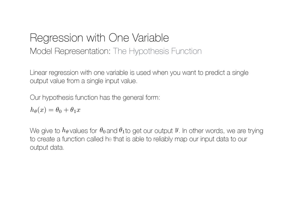
9. Regression with One Variable Model Representation: The Hypothesis Function Linear regression with one variable is used when you want to predict a single output value from a single input value. Our hypothesis function has the general form: We give to values for and to get our output . In other words, we are trying to create a function called hθ that is able to reliably map our input data to our output data. h✓( x ) = ✓0 + ✓1x ✓0 ✓1 y h✓
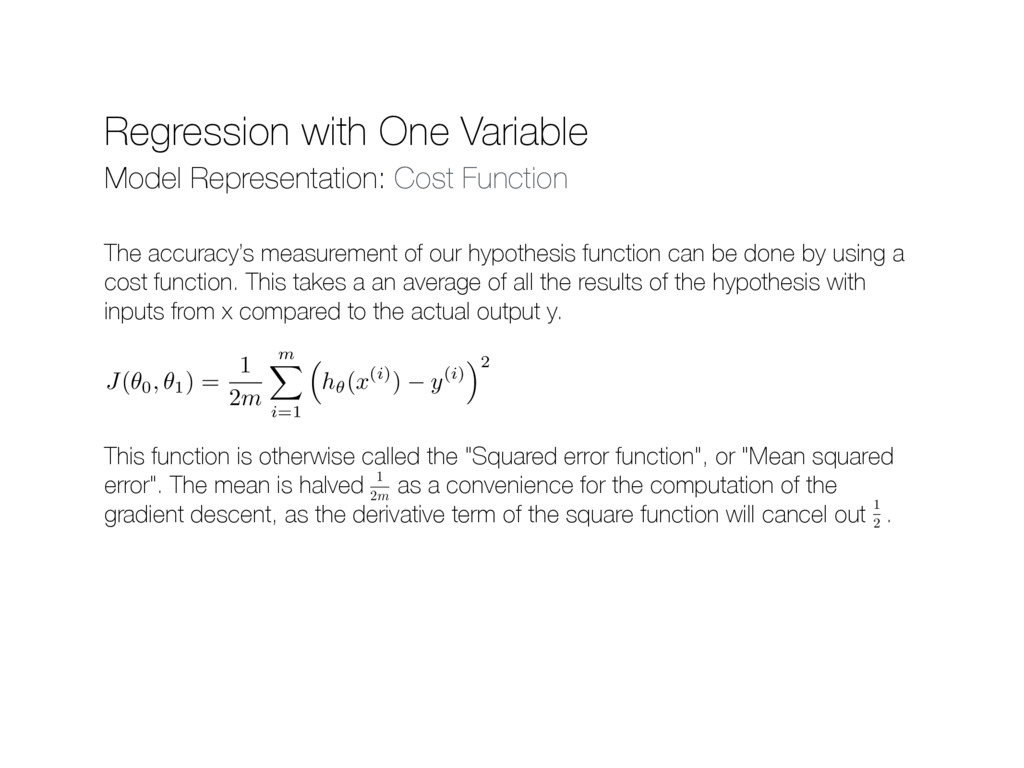
10. Regression with One Variable Model Representation: Cost Function The accuracy’s measurement of our hypothesis function can be done by using a cost function. This takes a an average of all the results of the hypothesis with inputs from x compared to the actual output y. This function is otherwise called the "Squared error function", or "Mean squared error". The mean is halved as a convenience for the computation of the gradient descent, as the derivative term of the square function will cancel out . J ( ✓0, ✓1) = 1 2 m m X i=1 ⇣ h✓( x (i)) y (i) ⌘2 1 2m 1 2
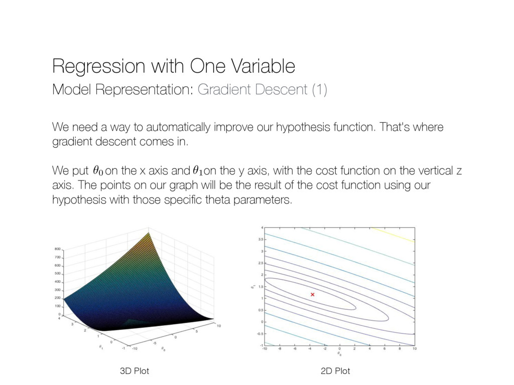
11. Regression with One Variable Model Representation: Gradient Descent (1) We need a way to automatically improve our hypothesis function. That's where gradient descent comes in. We put on the x axis and on the y axis, with the cost function on the vertical z axis. The points on our graph will be the result of the cost function using our hypothesis with those specific theta parameters. ✓0 ✓1 3D Plot 2D Plot
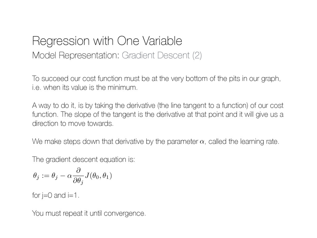
12. Regression with One Variable Model Representation: Gradient Descent (2) To succeed our cost function must be at the very bottom of the pits in our graph, i.e. when its value is the minimum. A way to do it, is by taking the derivative (the line tangent to a function) of our cost function. The slope of the tangent is the derivative at that point and it will give us a direction to move towards. We make steps down that derivative by the parameter , called the learning rate. The gradient descent equation is: for j=0 and i=1. You must repeat it until convergence. ↵ ✓j := ✓j ↵ @ @✓j J(✓0, ✓1)
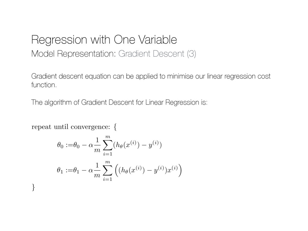
13. Regression with One Variable Model Representation: Gradient Descent (3) Gradient descent equation can be applied to minimise our linear regression cost function. The algorithm of Gradient Descent for Linear Regression is: ✓0 := ✓0 ↵ 1 m m X i=1 ( h✓( x (i)) y (i)) ✓1 := ✓1 ↵ 1 m m X i=1 ⇣ ( h✓( x (i)) y (i)) x (i) ⌘ repeat until convergence: { }
14. What can we do next? Instead of using linear regression on just one input variable, we can generalise and expand our concepts so that we can predict data with multiple input variables. Moreover, it exists another way to minimise the cost function: The Normal Equation. This method is numerical and not iterative (it means it takes only one step).