SER431 Lecture 16

Advanced Graphics
Cubic B-splines
(201810)

Transcript

1. jgs
   SER 431
   Advanced Graphics
   Lecture 16: B-spline Curves
   Javier Gonzalez-Sanchez
   javiergs@asu.edu
   PERALTA 230U
   Office Hours: By appointment
   

   View Slide

2. Javier Gonzalez-Sanchez | SER431 | Fall 2018 | 2
   jgs
   Problem 1
   § More control points higher the f(x) degree
   

   View Slide

3. Javier Gonzalez-Sanchez | SER431 | Fall 2018 | 3
   jgs
   Problem 2 | Continuity
   Definition of C0, C1, and C2 continuity
   

   View Slide

4. Javier Gonzalez-Sanchez | SER431 | Fall 2018 | 4
   jgs
   Problem 2 | Continuity
   § 2 Bezier with C0 continuity
   § 2 Bezier with C1 continuity
   § 2 Bezier with C2 continuity
   

   View Slide

5. Javier Gonzalez-Sanchez | SER431 | Fall 2018 | 5
   jgs
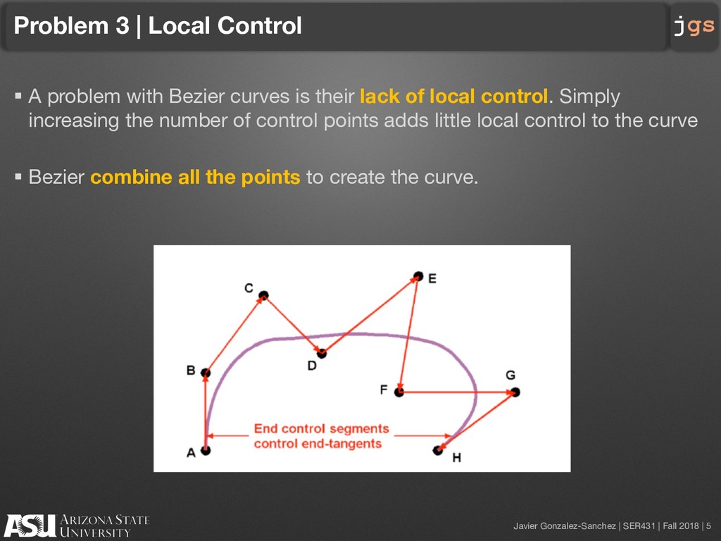
   Problem 3 | Local Control
   § A problem with Bezier curves is their lack of local control. Simply
   increasing the number of control points adds little local control to the curve
   § Bezier combine all the points to create the curve.
   

   View Slide

6. Javier Gonzalez-Sanchez | SER431 | Fall 2018 | 6
   jgs
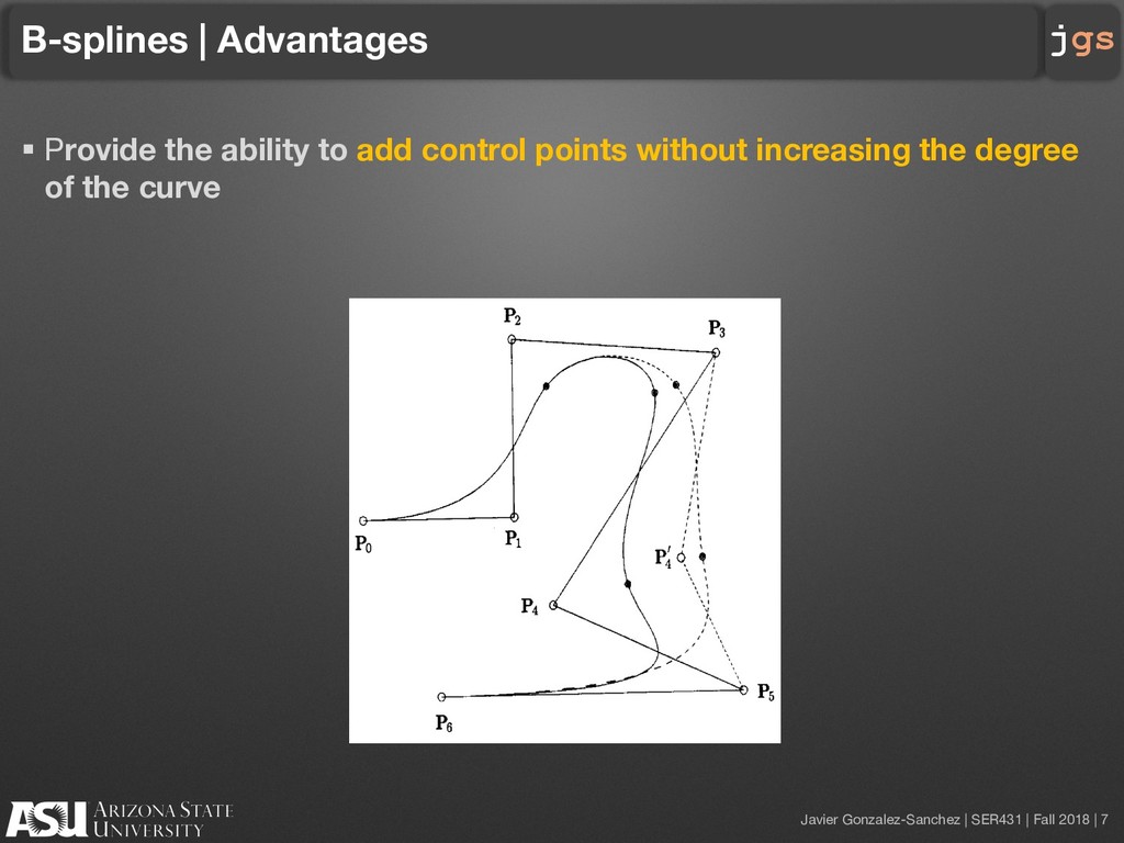
   B-splines
   § B-spline curves are powerful generalization of Bezier curves.
   § The B in B-spline stands for ”basis”.
   § B-spline segments are joined at knots. The blending functions uses a knot
   vector in every computation (instead of all of the control points)
   § When these knots are spaced evenly, the B-spline is said to be uniform,
   and non-uniform otherwise.
   

   View Slide

7. Javier Gonzalez-Sanchez | SER431 | Fall 2018 | 7
   jgs
   B-splines | Advantages
   § Provide the ability to add control points without increasing the degree
   of the curve
   

   View Slide

8. Javier Gonzalez-Sanchez | SER431 | Fall 2018 | 8
   jgs
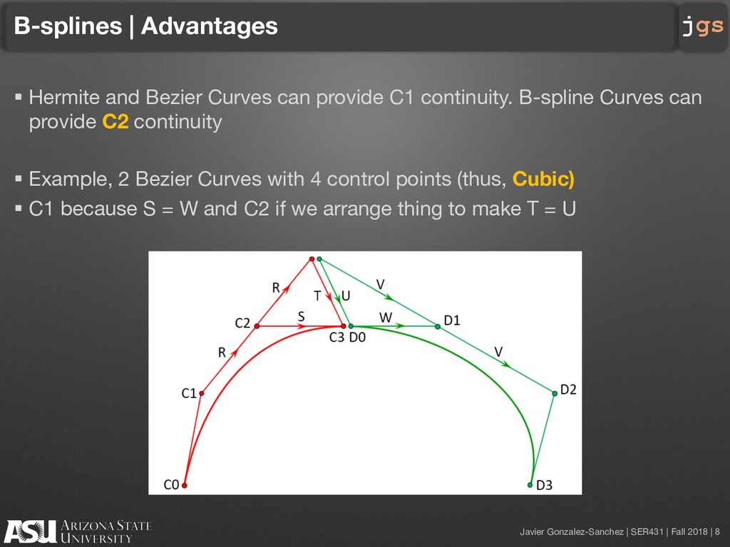
   B-splines | Advantages
   § Hermite and Bezier Curves can provide C1 continuity. B-spline Curves can
   provide C2 continuity
   § Example, 2 Bezier Curves with 4 control points (thus, Cubic)
   § C1 because S = W and C2 if we arrange thing to make T = U
   

   View Slide

9. Javier Gonzalez-Sanchez | SER431 | Fall 2018 | 9
   jgs
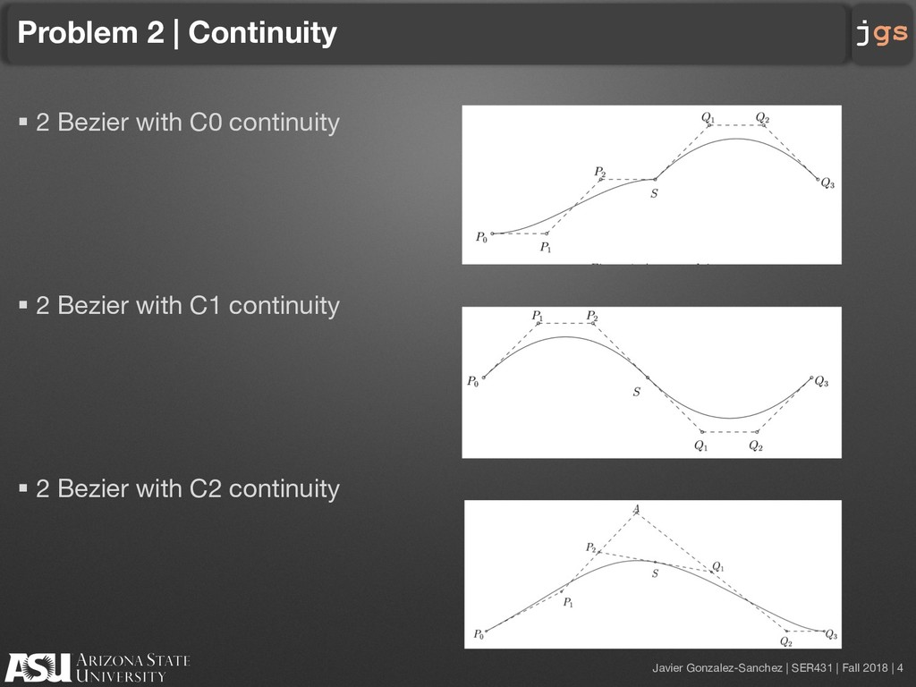
   If two Bezier curves are joined at a point S, both their first and second
   derivatives match at S (i.e., they are C2 continuous) if and only if their control
   polygons fit an A-Frame.
   

   View Slide

10. Javier Gonzalez-Sanchez | SER431 | Fall 2018 | 10
    jgs
    B-splines | Advantages
    § It combine only those points nearest to the current parameter.
    

    View Slide

11. Javier Gonzalez-Sanchez | SER431 | Fall 2018 | 11
    jgs
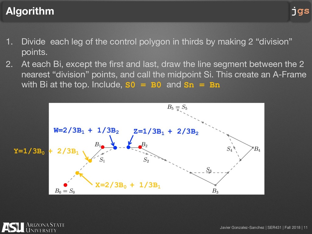
    Algorithm
    1. Divide each leg of the control polygon in thirds by making 2 “division”
    points.
    2. At each Bi, except the first and last, draw the line segment between the 2
    nearest “division” points, and call the midpoint Si. This create an A-Frame
    with Bi at the top. Include, S0 = B0 and Sn = Bn
    Y=1/3B0
    + 2/3B1
    X=2/3B0
    + 1/3B1
    W=2/3B1
    + 1/3B2 Z=1/3B1
    + 2/3B2
    

    View Slide

12. Javier Gonzalez-Sanchez | SER431 | Fall 2018 | 12
    jgs
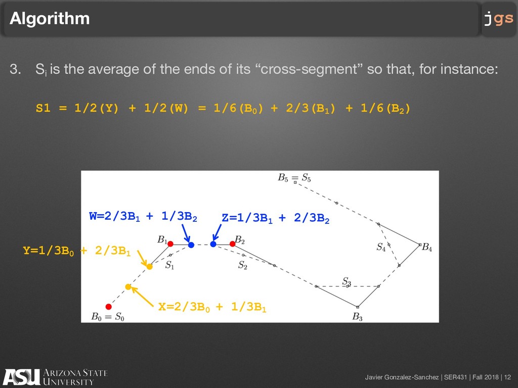
    Algorithm
    3. Si
    is the average of the ends of its “cross-segment” so that, for instance:
    S1 = 1/2(Y) + 1/2(W) = 1/6(B0
    ) + 2/3(B1
    ) + 1/6(B2
    )
    Y=1/3B0
    + 2/3B1
    X=2/3B0
    + 1/3B1
    W=2/3B1
    + 1/3B2 Z=1/3B1
    + 2/3B2
    

    View Slide

13. Javier Gonzalez-Sanchez | SER431 | Fall 2018 | 13
    jgs
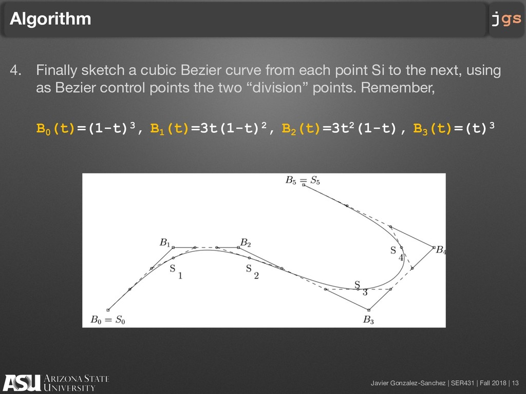
    Algorithm
    4. Finally sketch a cubic Bezier curve from each point Si to the next, using
    as Bezier control points the two “division” points. Remember,
    B0
    (t)=(1-t)3, B1
    (t)=3t(1-t)2, B2
    (t)=3t2(1-t), B3
    (t)=(t)3
    

    View Slide

14. jgs
    Source Code
    One Cubic B-spline curve
    

    View Slide

15. Javier Gonzalez-Sanchez | SER431 | Fall 2018 | 15
    jgs
    bspline.cpp
    § In red the control points
    § In yellow and blue the “division” points
    § In gray the Si
    midpoints
    SA
    SB
    

    View Slide

16. Javier Gonzalez-Sanchez | SER431 | Fall 2018 | 16
    jgs
    bspline.cpp
    float Points[4][3] = {
    { 10, 10, 0 },
    { 5, 10, 0 },
    { -5, 0, 0 },
    { -10, 5, 0 }
    };
    

    View Slide

17. Javier Gonzalez-Sanchez | SER431 | Fall 2018 | 17
    jgs
    bspline.cpp
    glColor3f(0, 1, 0);
    glBegin(GL_LINE_STRIP);
    for (int i = 0; i != N; ++i) {
    float t = (float)i / (N - 1);
    // the t value inverted
    float it = 1.0f - t;
    // calculate blending functions
    float b0 = it * it*it / 6.0f;
    float b1 = (3 * t*t*t - 6 * t*t + 4) / 6.0f;
    float b2 = (-3 * t*t*t + 3 * t*t + 3 * t + 1) / 6.0f;
    float b3 = t * t*t / 6.0f;
    // sum the control points mulitplied by their respective blending functions
    float x = b0*Points[0][0] + b1*Points[1][0] + b2*Points[2][0] + b3*Points[3][0];
    float y = b0*Points[0][1] + b1*Points[1][1] + b2*Points[2][1] + b3*Points[3][1];
    float z = b0*Points[0][2] + b1*Points[1][2] + b2*Points[2][2] + b3*Points[3][2];
    // draw
    glVertex3f(x, y, z);
    }
    glEnd();
    

    View Slide

18. jgs
    Source Code
    A collection of Cubic B-spline curves
    

    View Slide

19. Javier Gonzalez-Sanchez | SER431 | Fall 2018 | 19
    jgs
    bspline_connected.cpp
    § In red the control points
    § In yellow and blue the “division” points
    § In gray the Si
    midpoints
    SA
    SB
    

    View Slide

20. Javier Gonzalez-Sanchez | SER431 | Fall 2018 | 20
    jgs
    bspline.cpp
    float Points[7][3] = {
    { 10, 10, 0 },
    { 5, 10, 0 },
    { 0, 0, 0 },
    { -5, -5, 0 },
    {-10, 0, 0 },
    { -5, 10, 0 },
    { 0, 5, 0 }
    };
    #define NUM_POINTS 7
    #define NUM_SEGMENTS (NUM_POINTS+1)
    // curve segments to be draw
    // 0 0 0 1
    // 0 0 1 2
    // 0 1 2 3
    // 1 2 3 4
    // 2 3 4 5
    // 3 4 5 6
    // 4 5 6 6
    // 5 6 6 6
    0
    1
    2
    3
    4
    5
    6
    

    View Slide

21. Javier Gonzalez-Sanchez | SER431 | Fall 2018 | 21
    jgs
    bspline.cpp
    glBegin(GL_LINE_STRIP);
    float color=0;
    for (int segment = -3, j = 0; j != NUM_SEGMENTS; ++j, ++segment) {
    // for each section of curve, draw N divisions
    color = !color; glColor3f(color, 1, color);
    for (int i = 0; i != N; ++i) {
    float t = (float)i / N;
    float it = 1.0f - t;
    // calculate blending functions for cubic bspline.
    float b0 = it * it*it / 6.0f;
    float b1 = (3 * t*t*t - 6 * t*t + 4) / 6.0f;
    float b2 = (-3 * t*t*t + 3 * t*t + 3 * t + 1) / 6.0f;
    float b3 = t * t*t / 6.0f;
    // calculate the x,y and z of the curve point
    float x = b0 * GetPoint(segment + 0)[0] + b1 * GetPoint(segment + 1)[0] +
    b2 * GetPoint(segment + 2)[0] + b3 * GetPoint(segment + 3)[0];
    float y = b0 * GetPoint(segment + 0)[1] + b1 * GetPoint(segment + 1)[1] +
    b2 * GetPoint(segment + 2)[1] + b3 * GetPoint(segment + 3)[1];
    float z = b0 * GetPoint(segment + 0)[2] + b1 * GetPoint(segment + 1)[2] +
    b2 * GetPoint(segment + 2)[2] + b3 * GetPoint(segment + 3)[2];
    // specify the point.
    glVertex3f(x, y, z);
    }
    

    View Slide

22. Javier Gonzalez-Sanchez | SER431 | Fall 2018 | 22
    jgs
    bspline.cpp
    }
    // specify the last point on the curve
    glVertex3fv(Points[NUM_POINTS - 1]);
    glEnd();
    

    View Slide

23. Javier Gonzalez-Sanchez | SER431 | Fall 2018 | 23
    jgs
    Test Yourselves
    § Modify the code in GitHub to draw the following B-splines
    23
    

    View Slide

24. Javier Gonzalez-Sanchez | SER431 | Fall 2018 | 24
    jgs
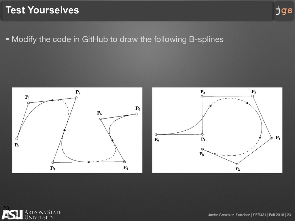
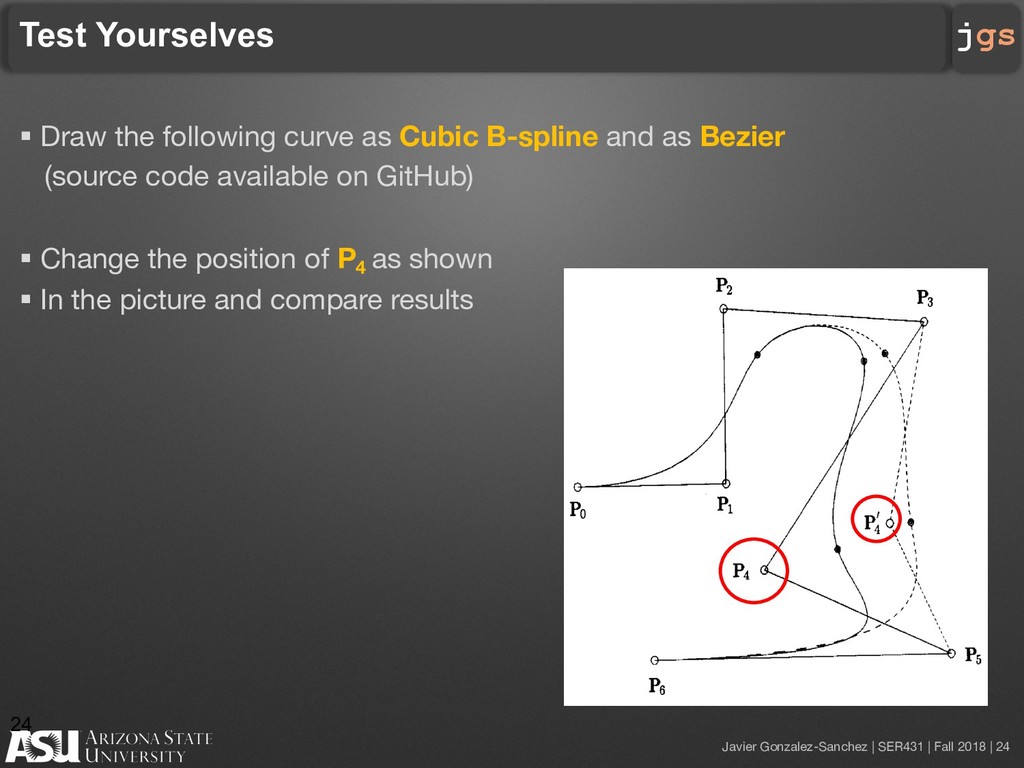
    Test Yourselves
    § Draw the following curve as Cubic B-spline and as Bezier
    (source code available on GitHub)
    § Change the position of P
    4
    as shown
    § In the picture and compare results
    24
    

    View Slide

25. jgs
    SER431 Advanced Graphics
    Javier Gonzalez-Sanchez
    javiergs@asu.edu
    Fall 2018
    Disclaimer. These slides can only be used as study material for the class SER431 at ASU. They cannot be
    distributed or used for another purpose.
    

    View Slide