Bayesian inference of effective contagion models from population level data

Flash talk at SINM 2019 (http://danlarremore.com/sinm2019/)

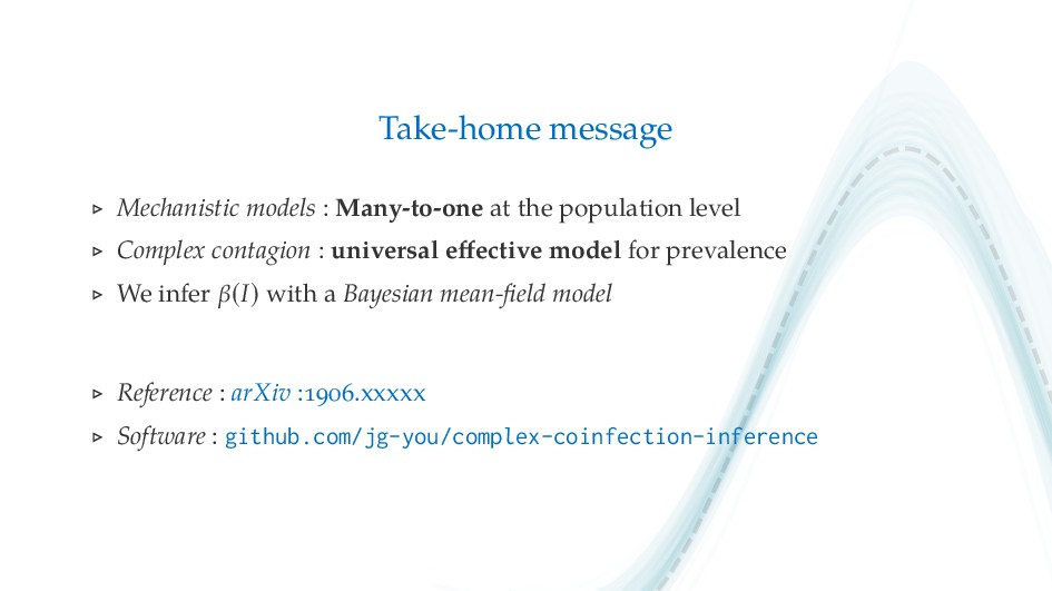
Preprint: https://arxiv.org/abs/1906.01147
Software: https://github.com/jg-you/complex-coinfection-inference/

See also: "Interacting simple contagions are complex contagions," by Laurent Hébert-Dufresne: https://speakerdeck.com/laurenthebert/interacting-simple-contagions-are-complex-contagions

Extended abstract
==============
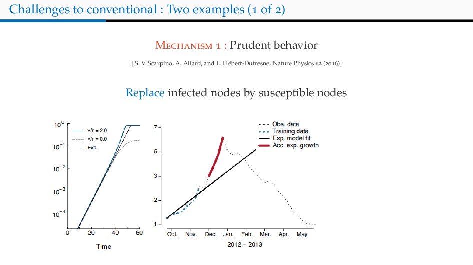
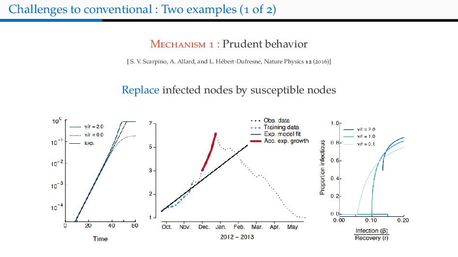
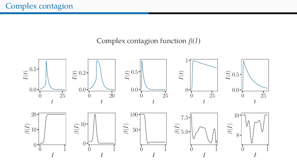
Contagions never occur in a vacuum. Instead, diseases and ideas interact with each other and with externalities such as host connectivity, behaviour, and mobility. Several recent studies have shown that many of these non-linear mechanism lead to rich dynamics that can exhibit, for example, a non-monotonous relation between the expected epidemic size and their average transmission rate and discontinuous phase transitions. Surprisingly, many of these features arise from minor alterations to the mechanistic rules of the models. In other words, innocuous looking modeling choices can produce drastically different outcomes that would lead to very different conclusions about intervention strategies or risk. Understanding how to properly generalize contagion models is, as a result, perhaps one of the most pressing challenge of network epidemiology.

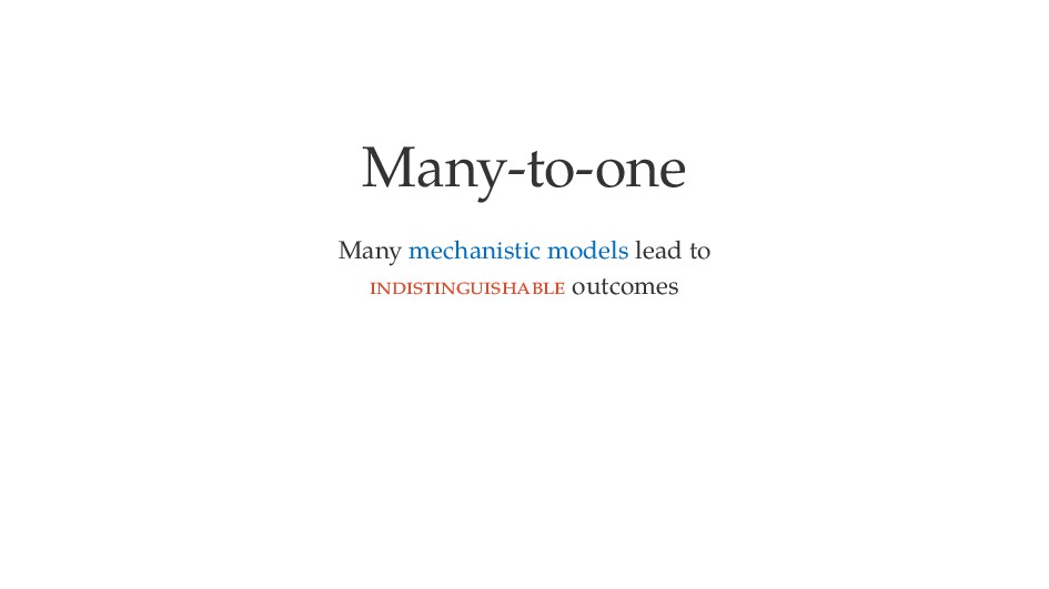
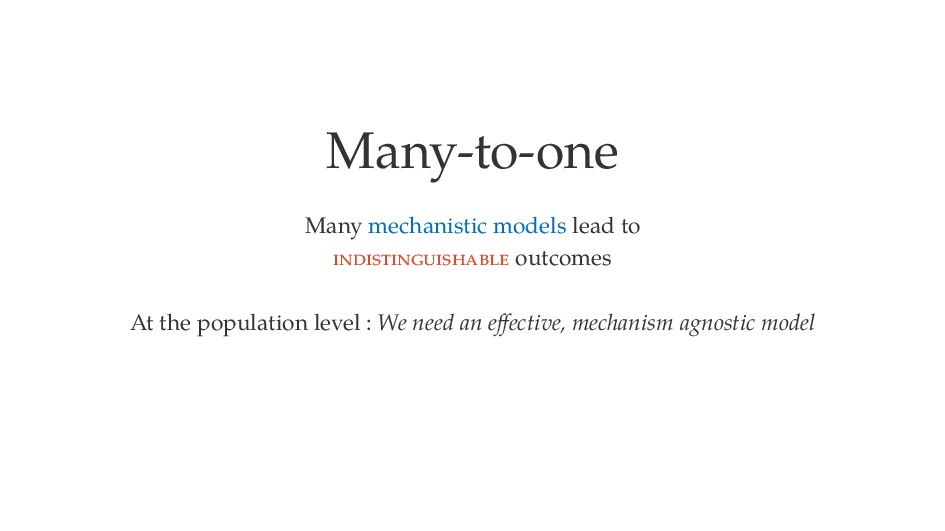
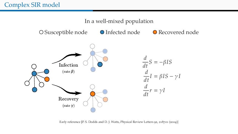
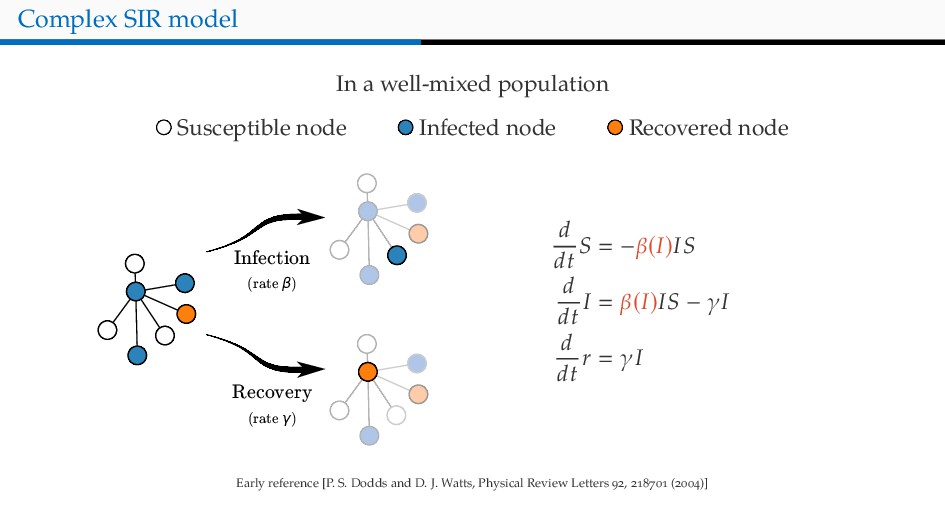
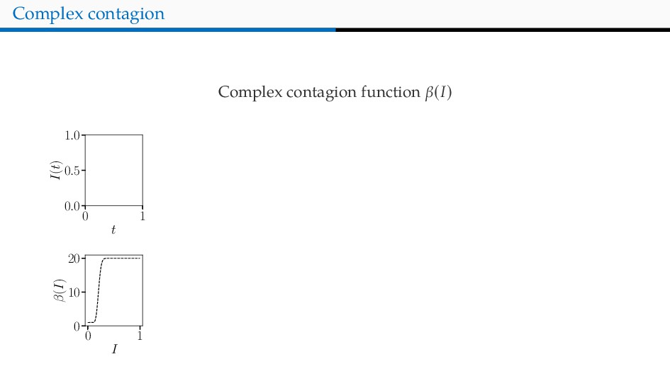
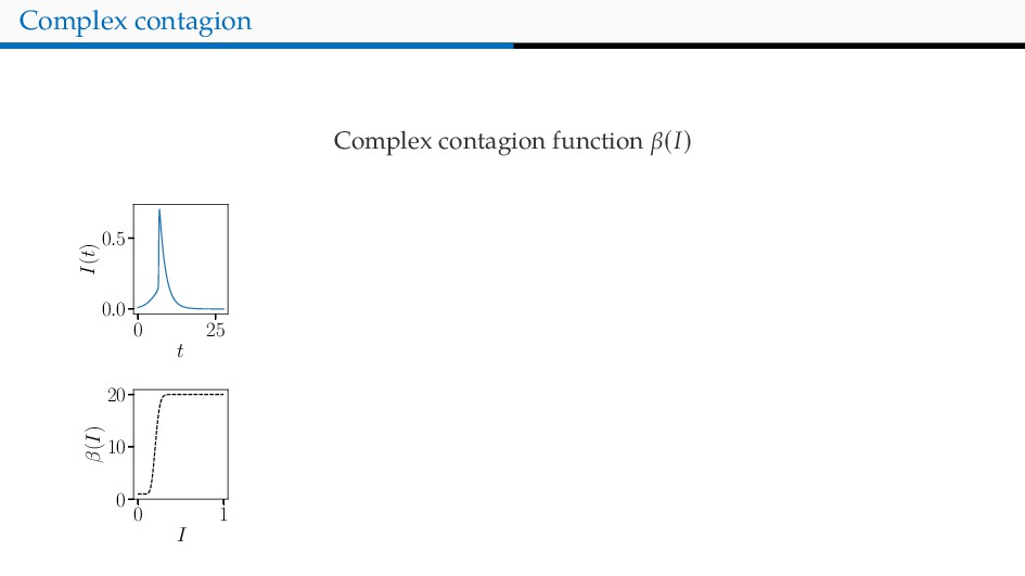
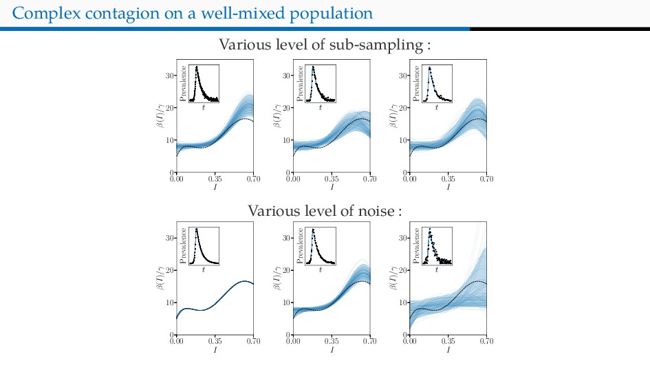
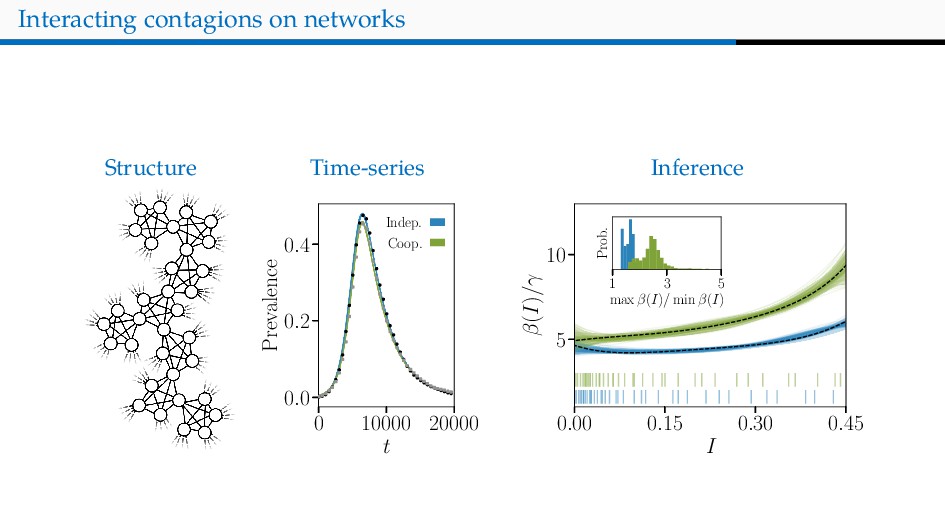
Recent work shows that so-called “complex contagions models” can induce many of the defining features of the new wave of non-linear mechanistic models. Complex contagion models achieve this by modifying the transmission rate β(I), as to let it depend on the density of infected individuals in the neighbourhood of the susceptible individuals. In this work, we show that some complex contagion models are in fact indistinguishable from a number of non-linear mechanistic models at the population level. This motivates us to think of complex contagion (on Erdős-Rényi graphs) as a useful effective model of contagion on networks. The complex contagion function β(I) that appears in this model captures arbitrary non-linear effects, allowing us to the contagions without making any mechanistic assumptions. By understanding how mechanistic models map unto this complex contagion model, we can interpret the function β(I) and draw tentative inference about the population under scrutiny.

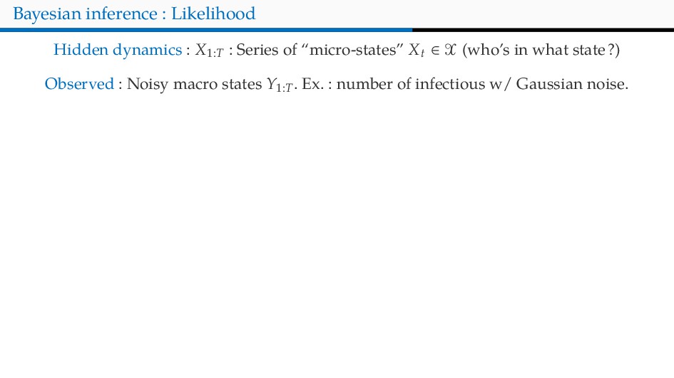
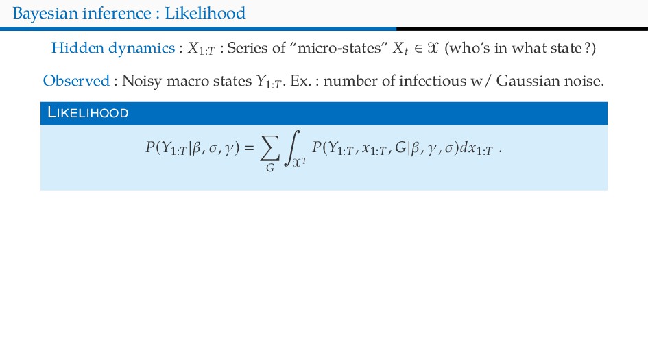
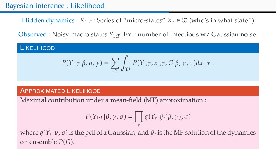
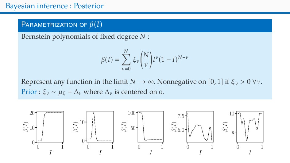
We develop a fully Bayesian method to fit our effective contagion model to population-level data. This allows us to infer posterior distributions of: Potential epidemiological trajectory, complex contagion functions β(I), and noise components. We avoid overfitting—a problem that arises in related approaches—by parameterizing the complex contagion functions as low degree polynomials. The net results is a flexible, efficient, yet expressive model that can be easily fitted to real and synthetic data alike.

Transcript

1. B
   SINM : F
   Jean-Gabriel Young
   Center for the Study of Complex Systems, University of Michigan, Ann Arbor, MI, USA
   jgyoung.ca @_jgyou
   May th,
   Based on joint work with Laurent Hébert-Dufresne and Samuel V. Scarpino
   

   View Slide

2. 1998
   1999
   2000
   2001
   2002
   2003
   2004
   2005
   2006
   2007
   2008
   2009
   2010
   2011
   2012
   2013
   2014
   0.0
   2.5
   5.0
   7.5
   New cases (% national)
   National Influenza data, CDC FluView Portal (WHO & ILINet)
   

   View Slide

3. At the population level : a longstanding approach
   Compartmental modeling, e.g. :
   Susceptible node Infected node Recovered node
   Infection
   (rate β)
   Recovery
   (rate γ)
   d
   dt
   S −βIS
   d
   dt
   I βIS − γI
   d
   dt
   r γI
   

   View Slide

4. At the population level : a longstanding approach
   Well-mixed
   0 10 20
   t
   10−2
   10−1
   100
   Densities
   I(t)
   R(t)
   Heterogeneous
   networks
   0 10 20
   t
   10−2
   10−1
   100
   Densities
   I(t)
   R(t)
   

   View Slide

5. Challenges to conventional : Two examples ( of )
   M : Prudent behavior
   [ S. V. Scarpino, A. Allard, and L. Hébert-Dufresne, Nature Physics ( )]
   Replace infected nodes by susceptible nodes
   

   View Slide

6. Challenges to conventional : Two examples ( of )
   M : Prudent behavior
   [ S. V. Scarpino, A. Allard, and L. Hébert-Dufresne, Nature Physics ( )]
   Replace infected nodes by susceptible nodes
   

   View Slide

7. Challenges to conventional wisdom : Two examples ( of )
   M : Interaction in clustered networks
   [ L. Hébert-Dufresne, S. V. Scarpino, and JGY (in preparation)]
   T diseases in well-mixed populations. Nodes with both become superspreaders.
   

   View Slide

8. Many-to-one
   Many mechanistic models lead to
   outcomes
   

   View Slide

9. Many-to-one
   Many mechanistic models lead to
   outcomes
   At the population level : We need an effective, mechanism agnostic model
   

   View Slide

10. Complex SIR model
    In a well-mixed population
    Susceptible node Infected node Recovered node
    Infection
    (rate β)
    Recovery
    (rate γ)
    d
    dt
    S −βIS
    d
    dt
    I βIS − γI
    d
    dt
    r γI
    Early reference [P. S. Dodds and D. J. Watts, Physical Review Letters , ( )]
    

    View Slide

11. Complex SIR model
    In a well-mixed population
    Susceptible node Infected node Recovered node
    Infection
    (rate β)
    Recovery
    (rate γ)
    d
    dt
    S −β(I)IS
    d
    dt
    I β(I)IS − γI
    d
    dt
    r γI
    Early reference [P. S. Dodds and D. J. Watts, Physical Review Letters , ( )]
    

    View Slide

12. Complex contagion
    Complex contagion function β(I)
    0 1
    t
    0.0
    0.5
    1.0
    I(t)
    0 1
    I
    0
    10
    20
    β(I)
    

    View Slide

13. Complex contagion
    Complex contagion function β(I)
    0 25
    t
    0.0
    0.5
    I(t)
    0 1
    I
    0
    10
    20
    β(I)
    

    View Slide

14. Complex contagion
    Complex contagion function β(I)
    0 25
    t
    0.0
    0.5
    I(t)
    0 1
    I
    0
    10
    20
    β(I)
    0 20
    t
    0.0
    0.2
    I(t)
    0 1
    I
    0
    10
    β(I)
    0 25
    t
    0.0
    0.5
    I(t)
    0 1
    I
    50
    100
    β(I)
    0 25
    t
    0
    1
    I(t)
    0 1
    I
    5.0
    7.5
    β(I)
    0 25
    t
    0.0
    0.5
    I(t)
    0 1
    I
    8
    10
    β(I)
    

    View Slide

15. I
    

    View Slide

16. Bayesian inference : Likelihood
    Hidden dynamics : X1:T : Series of “micro-states” Xt
    ∈ X(who’s in what state?)
    Observed : Noisy macro states Y1:T. Ex. : number of infectious w/ Gaussian noise.
    

    View Slide

17. Bayesian inference : Likelihood
    Hidden dynamics : X1:T : Series of “micro-states” Xt
    ∈ X(who’s in what state?)
    Observed : Noisy macro states Y1:T. Ex. : number of infectious w/ Gaussian noise.
    L
    P(Y1:T
    |β, σ, γ)
    G
    ∫
    XT
    P(Y1:T
    , x1:T
    , G|β, γ, σ)dx1:T
    .
    

    View Slide

18. Bayesian inference : Likelihood
    Hidden dynamics : X1:T : Series of “micro-states” Xt
    ∈ X(who’s in what state?)
    Observed : Noisy macro states Y1:T. Ex. : number of infectious w/ Gaussian noise.
    L
    P(Y1:T
    |β, σ, γ)
    G
    ∫
    XT
    P(Y1:T
    , x1:T
    , G|β, γ, σ)dx1:T
    .
    A
    Maximal contribution under a mean-field (MF) approximation :
    P(Y1:T
    |β, γ, σ)
    t
    q(Yt
    | ˜
    yt
    (β, γ), σ)
    where q(Yt
    |y, σ) is the pdf of a Gaussian, and ˜
    yt is the MF solution of the dynamics
    on ensemble P(G).
    

    View Slide

19. I
    

    View Slide

20. Complex contagion on a well-mixed population
    Various level of sub-sampling :
    0.00 0.35 0.70
    I
    0
    10
    20
    30
    β(I)/γ
    t
    Prevalence
    0.00 0.35 0.70
    I
    0
    10
    20
    30
    β(I)/γ
    t
    Prevalence
    0.00 0.35 0.70
    I
    0
    10
    20
    30
    β(I)/γ
    t
    Prevalence
    Various level of noise :
    0.00 0.35 0.70
    I
    0
    10
    20
    30
    β(I)/γ
    t
    Prevalence
    0.00 0.35 0.70
    I
    0
    10
    20
    30
    β(I)/γ
    t
    Prevalence
    0.00 0.35 0.70
    I
    0
    10
    20
    30
    β(I)/γ
    t
    Prevalence
    

    View Slide

21. Interacting contagions on networks
    Structure Time-series Inference
    0 10000 20000
    t
    0.0
    0.2
    0.4
    Prevalence
    Indep.
    Coop.
    0.00 0.15 0.30 0.45
    I
    5
    10
    β(I)/γ
    1 3 5
    max β(I)/ min β(I)
    Prob.
    

    View Slide

22. Reference : arXiv : .xxxxx
    Code : github.com/jg-you/comp ex-coinfection-inference
    jgyou@umich.edu jgyoung.ca @_jgyou
    

    View Slide

23. Take-home message
    Mechanistic models : Many-to-one at the population level
    Complex contagion : universal effective model for prevalence
    We infer β(I) with a Bayesian mean-field model
    Reference : arXiv : .xxxxx
    Software : github.com/jg-you/comp ex-coinfection-inference
    

    View Slide

24. View Slide

25. Bayesian inference : Posterior
    P β(I)
    Bernstein polynomials of fixed degree N :
    β(I)
    N
    ν 0
    ξν
    N
    ν
    Iν(1 − I)N−ν
    Represent any function in the limit N → ∞. Nonnegative on [0, 1] if ξν > 0 ∀ν.
    Prior : ξν ∼ µξ + ∆ν where ∆ν is centered on .
    0 25
    t
    0.0
    0.5
    I(t)
    0 1
    I
    0
    10
    20
    β(I)
    0 20
    t
    0.0
    0.2
    I(t)
    0 1
    I
    0
    10
    β(I)
    0 25
    t
    0.0
    0.5
    I(t)
    0 1
    I
    50
    100
    β(I)
    0 25
    t
    0
    1
    I(t)
    0 1
    I
    5.0
    7.5
    β(I)
    0 25
    t
    0.0
    0.5
    I(t)
    0 1
    I
    8
    10
    β(I)
    

    View Slide