Construction of and efficient sampling from the simplicial configuration model

Presented at HONS 2017 (http://complexdata.businesscatalyst.com/2017/)

Paper: https://doi.org/10.1103/PhysRevE.96.032312
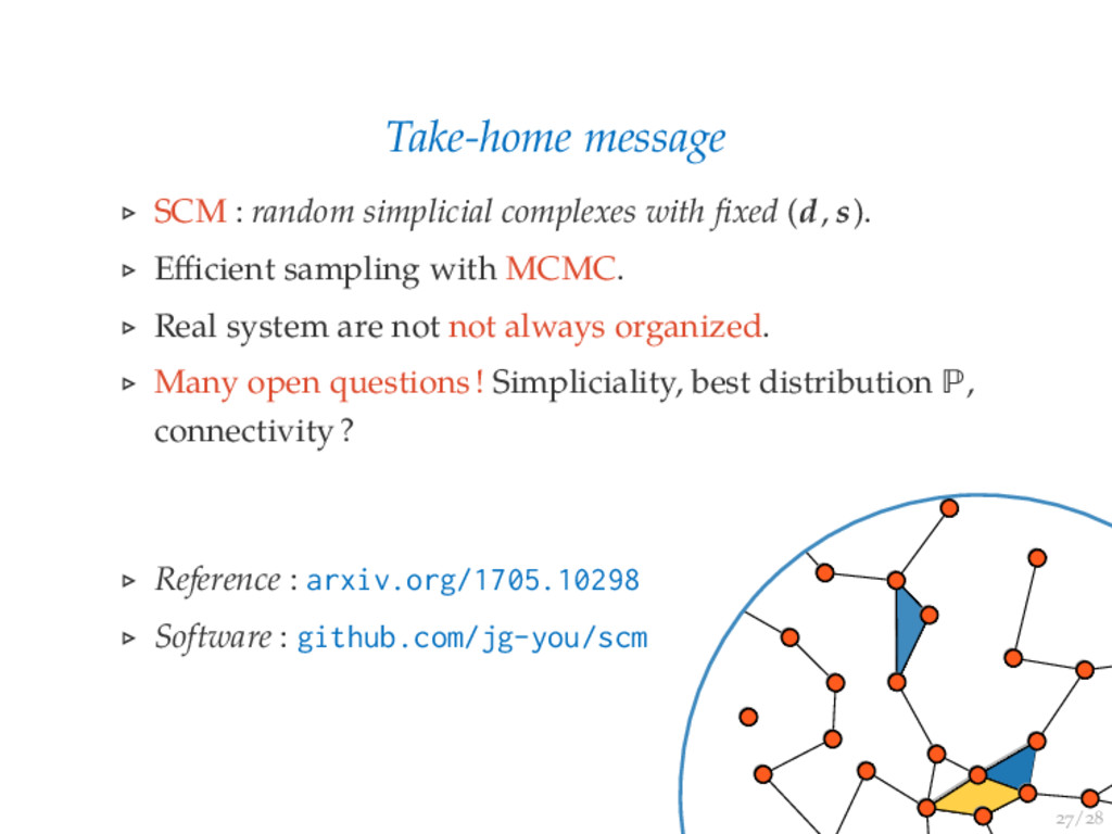
arXiv: https://arxiv.org/abs/1705.10298
Code: https://github.com/jg-you/scm/

Abstract
=======
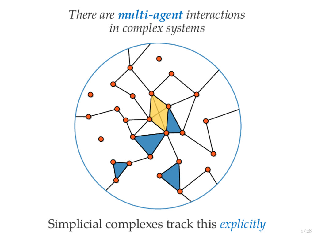
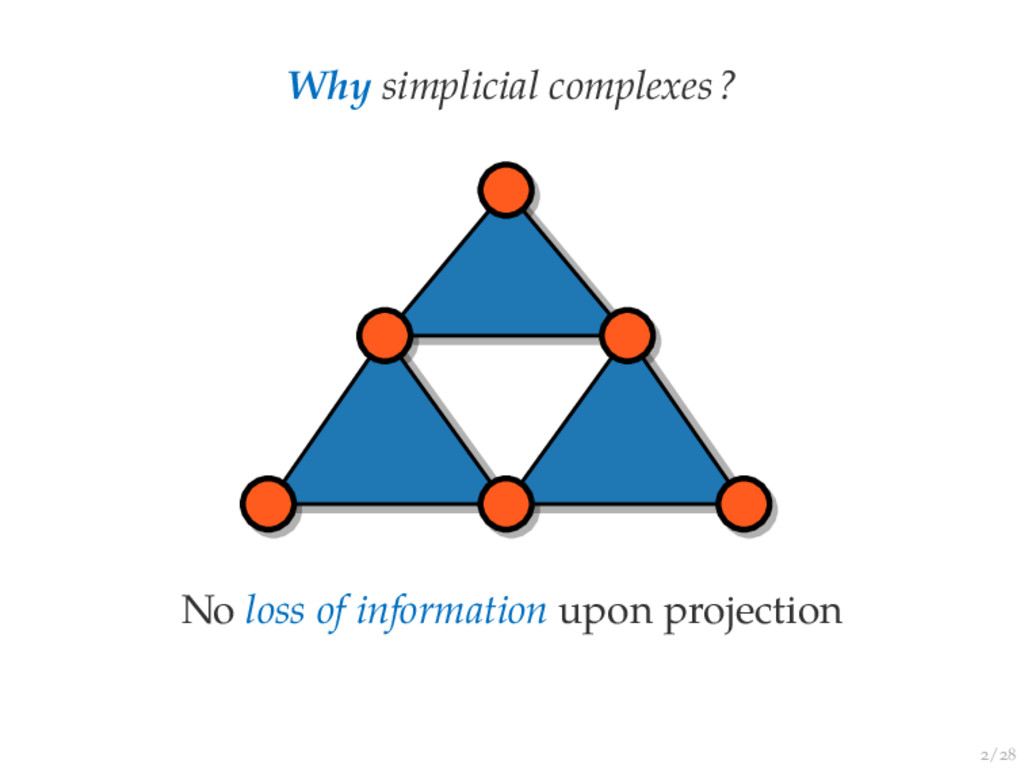
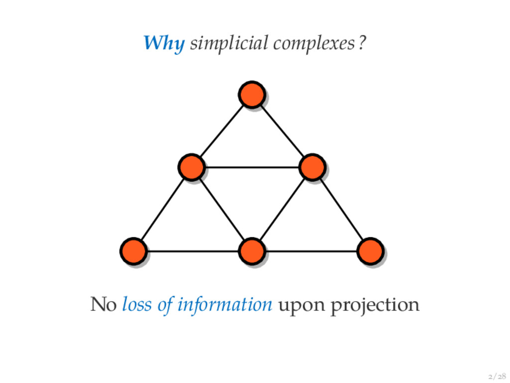
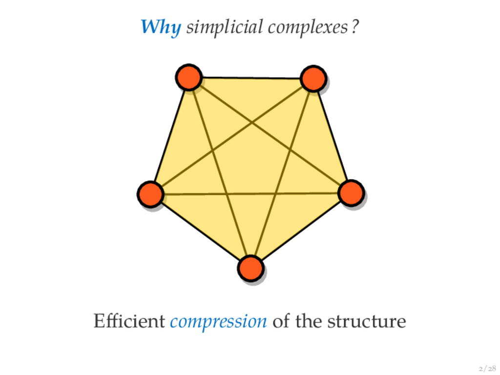
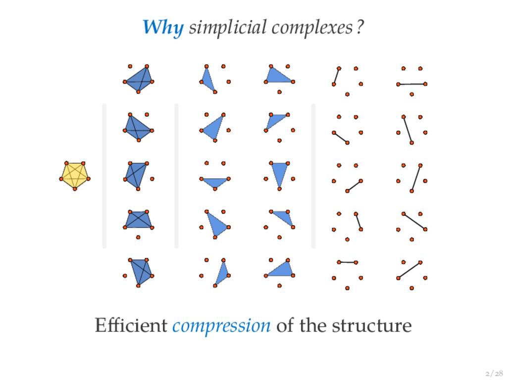
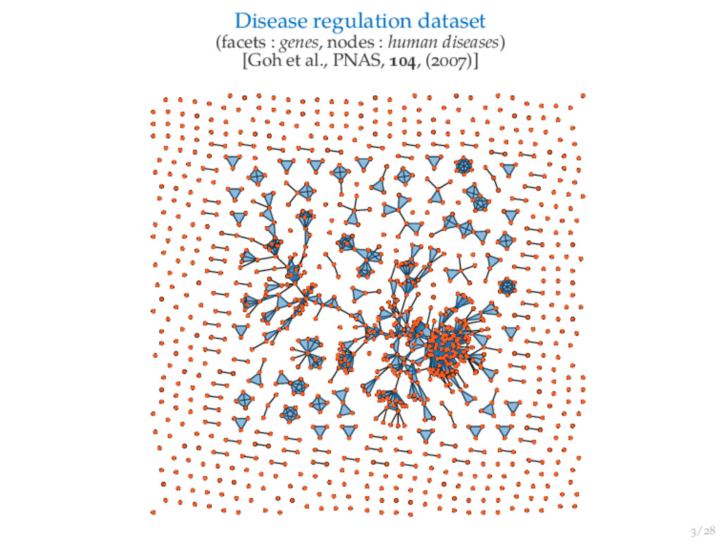
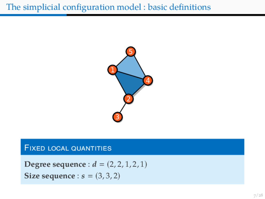
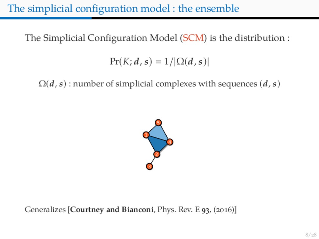
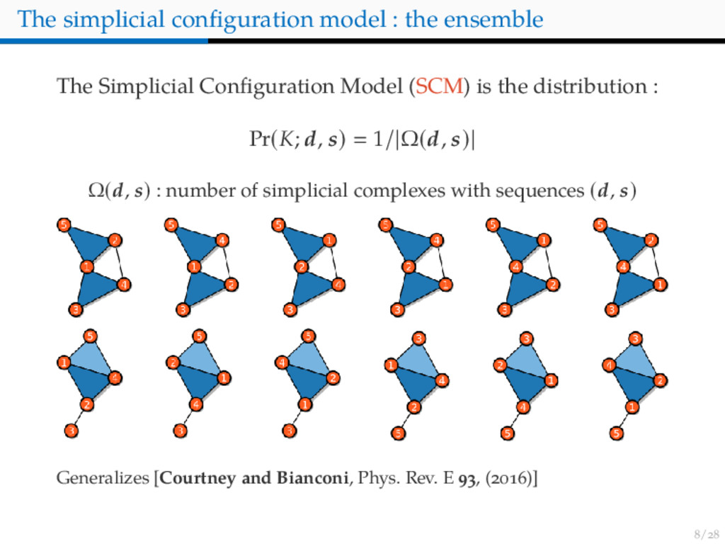
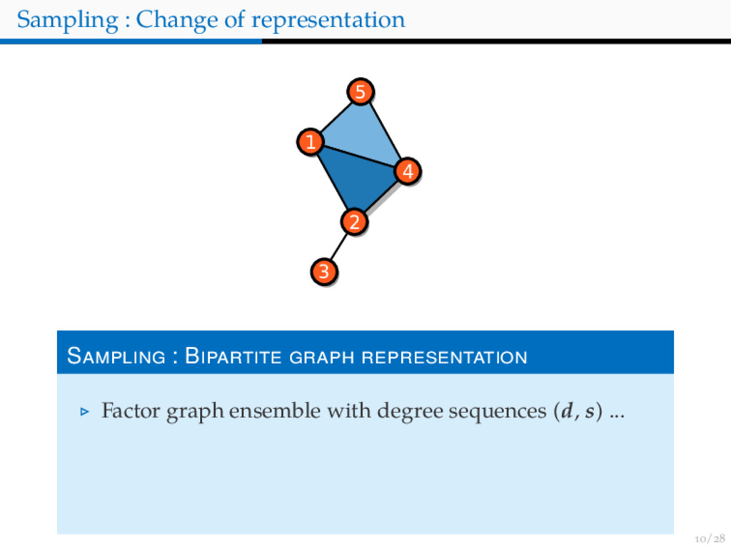
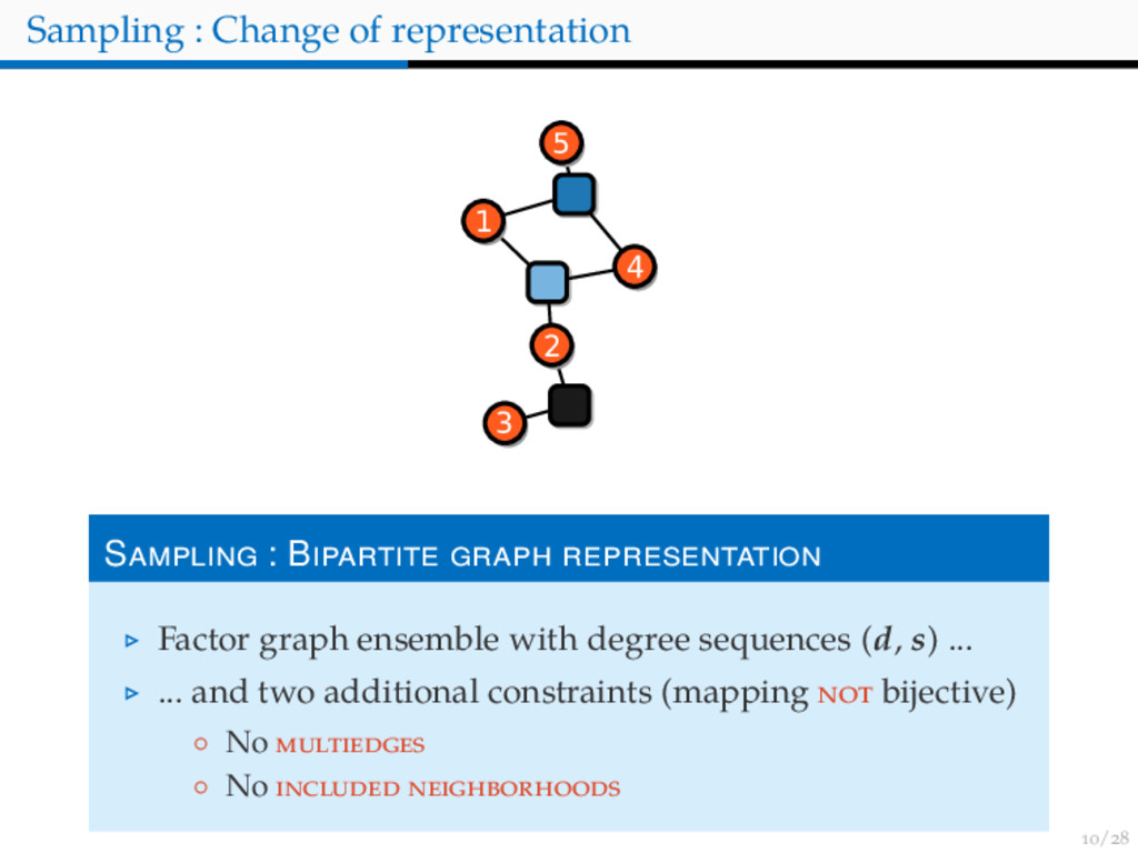
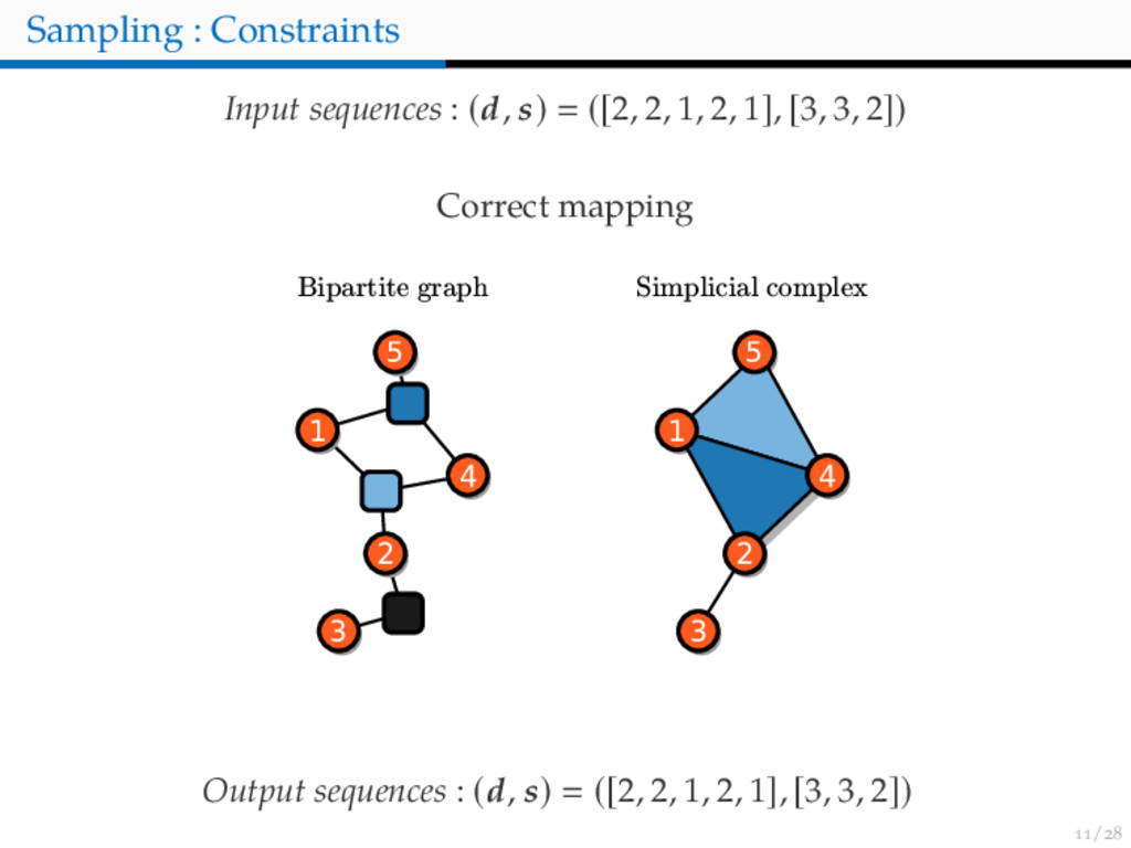
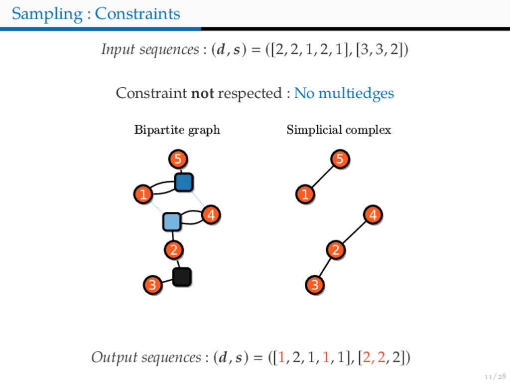
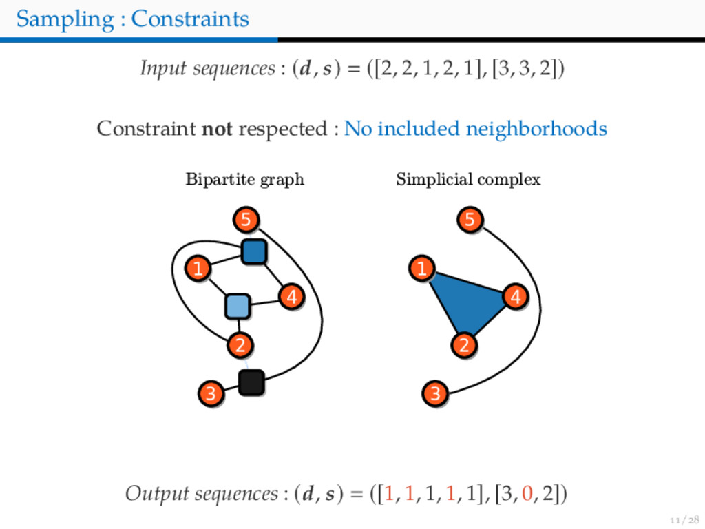
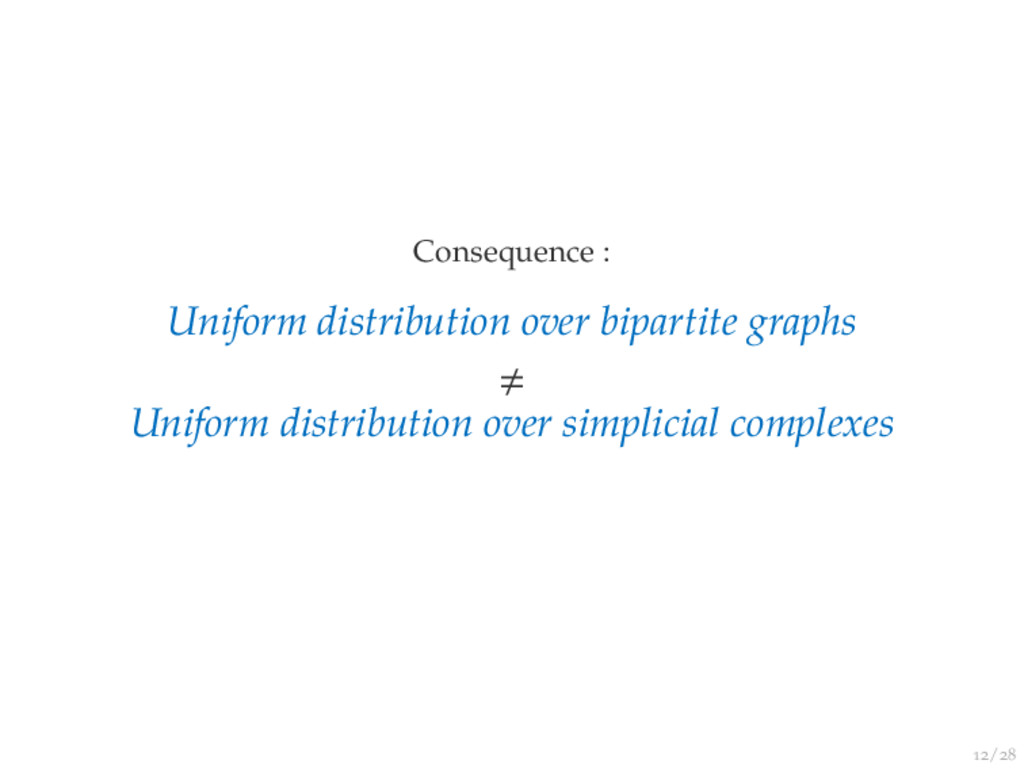
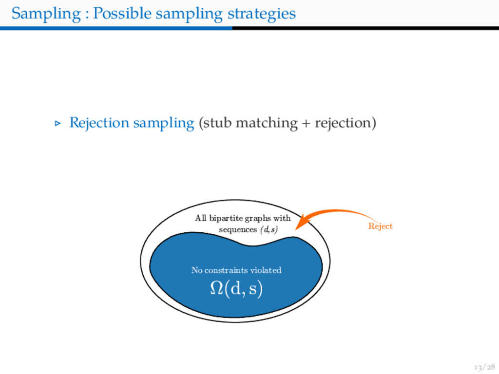
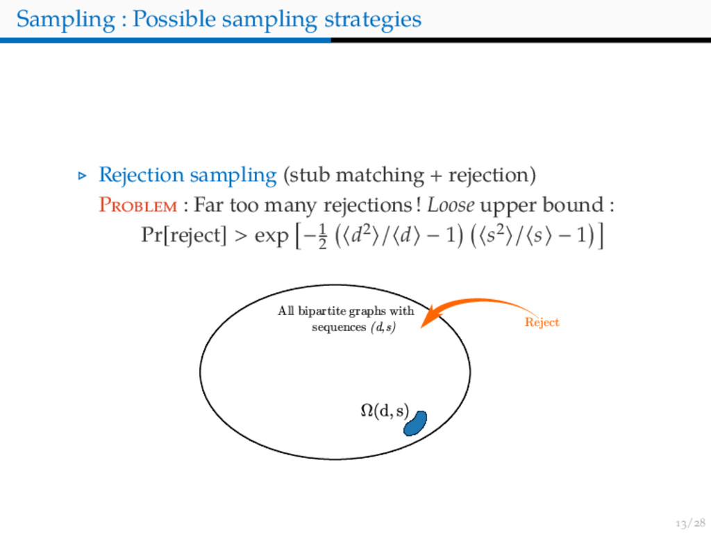
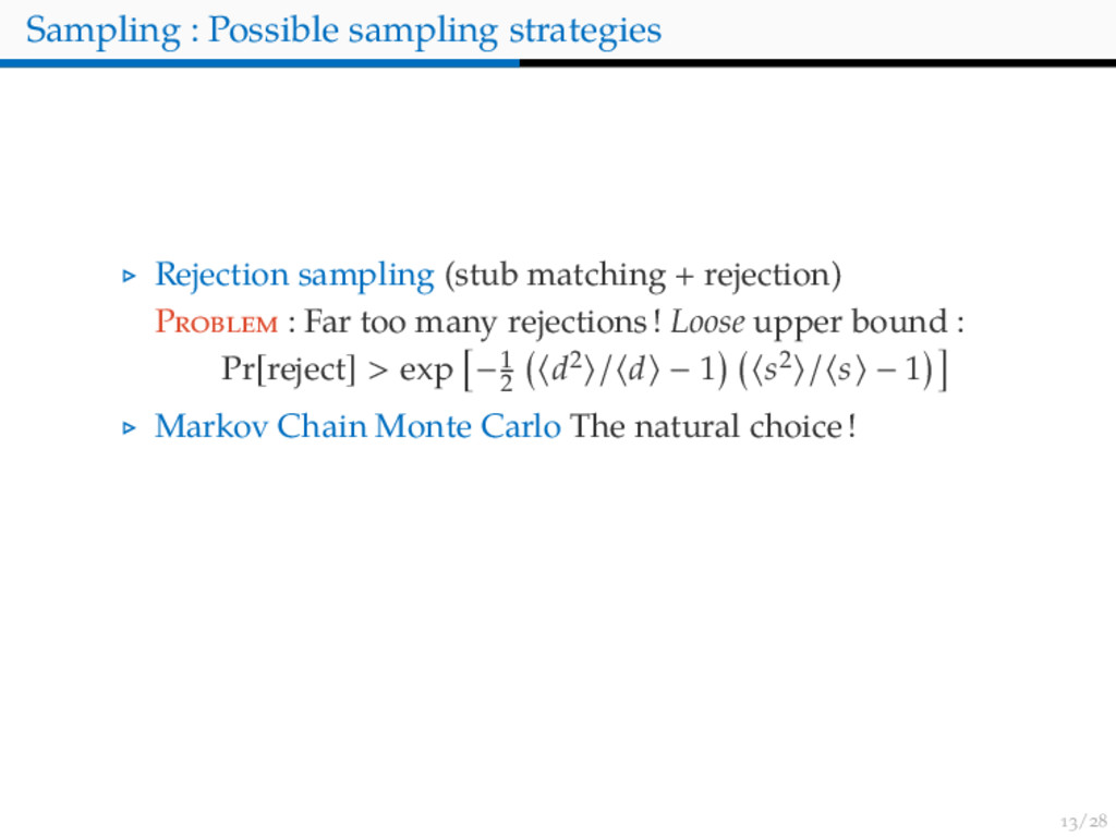
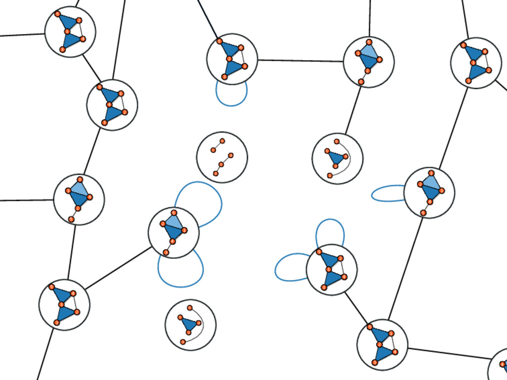
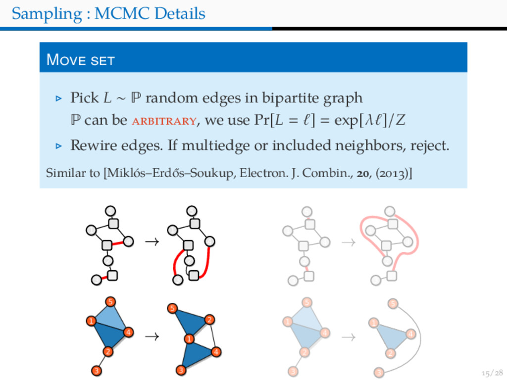
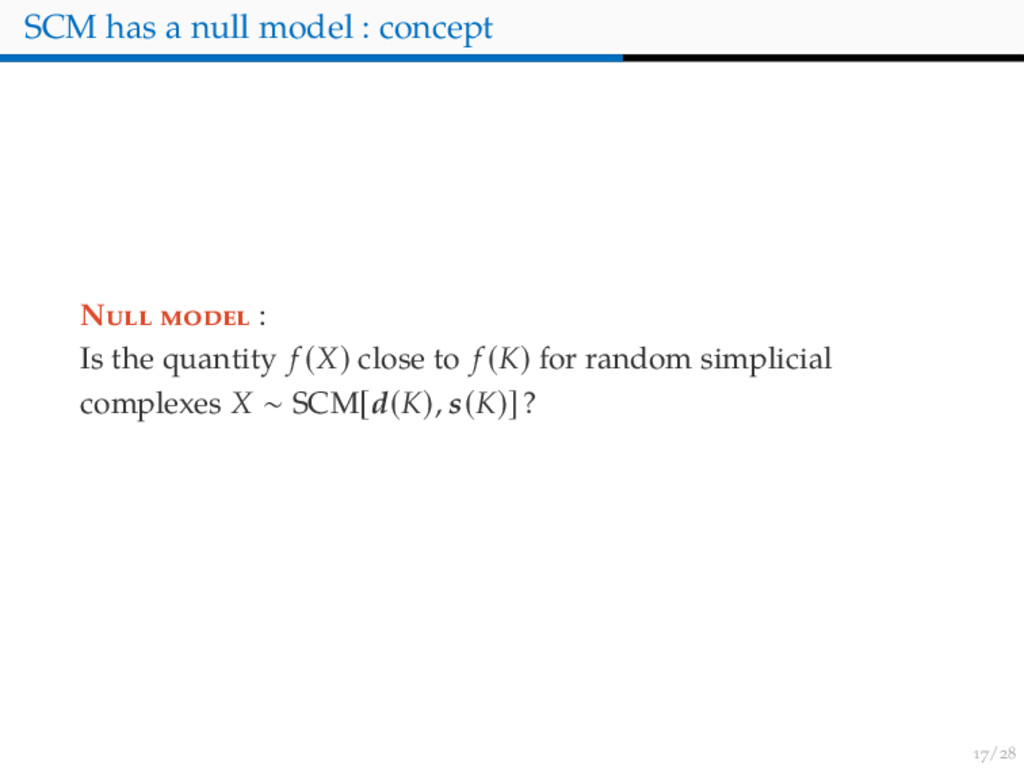
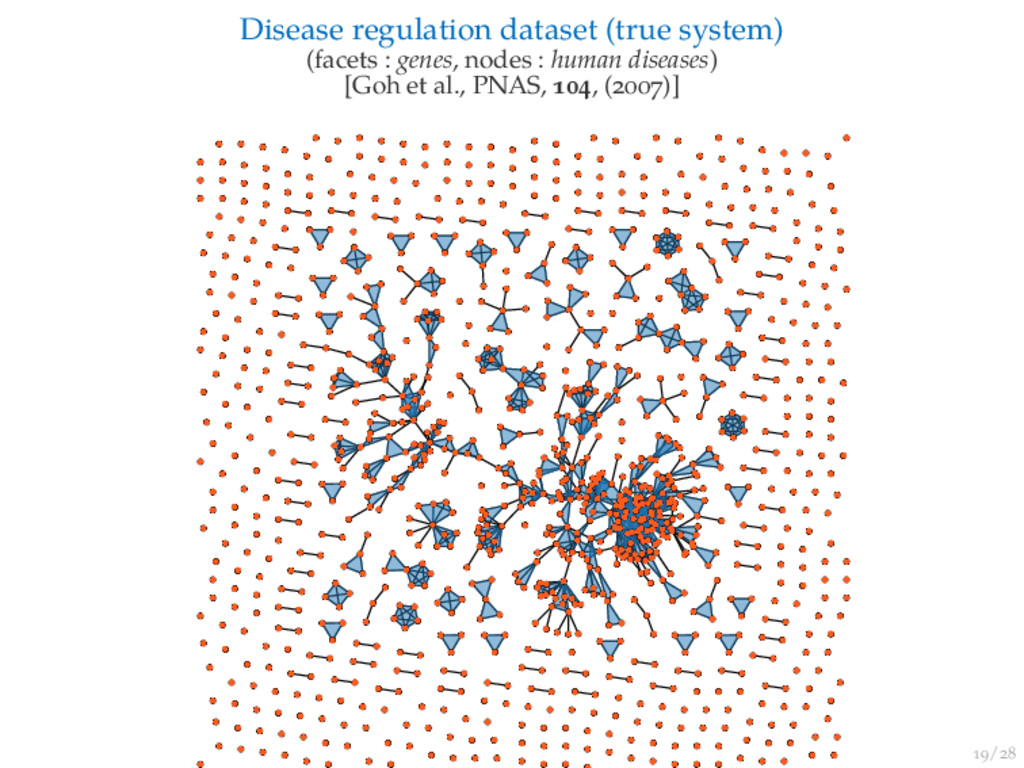
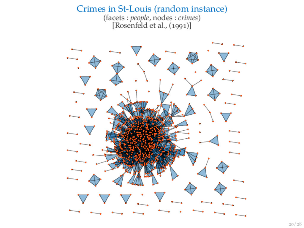
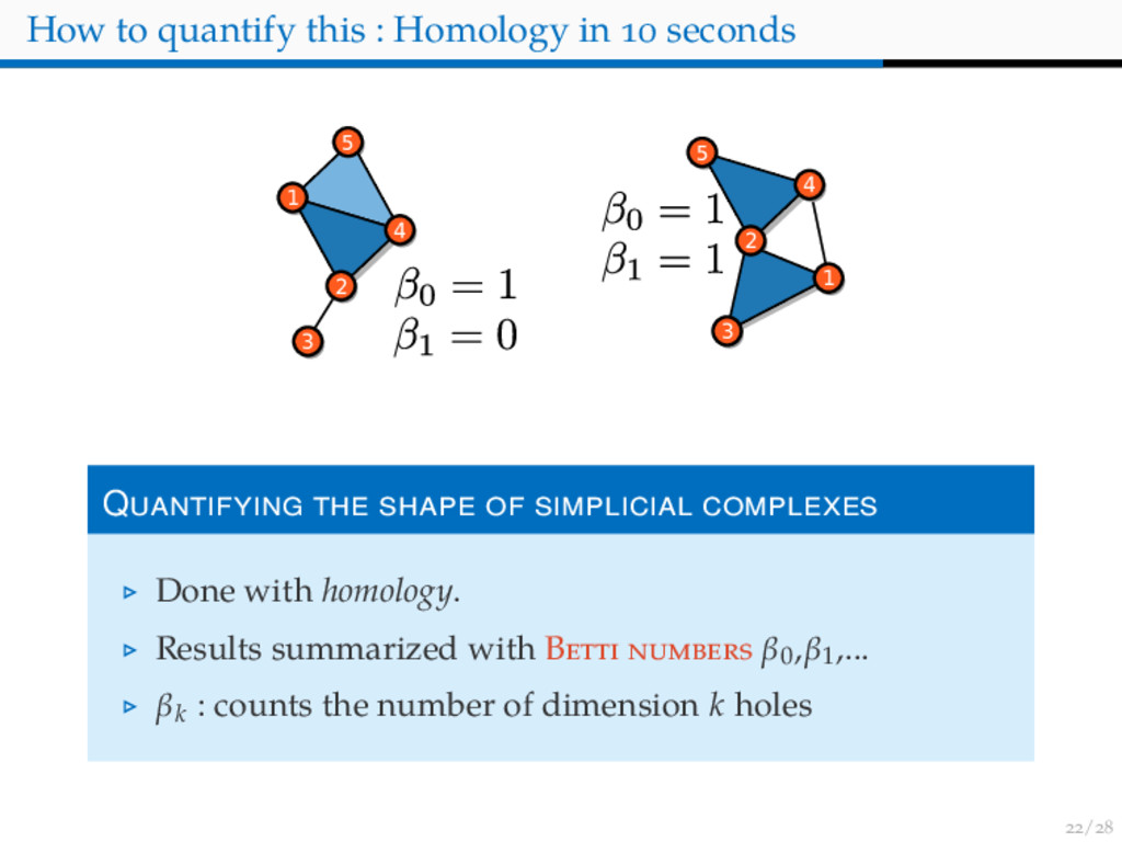
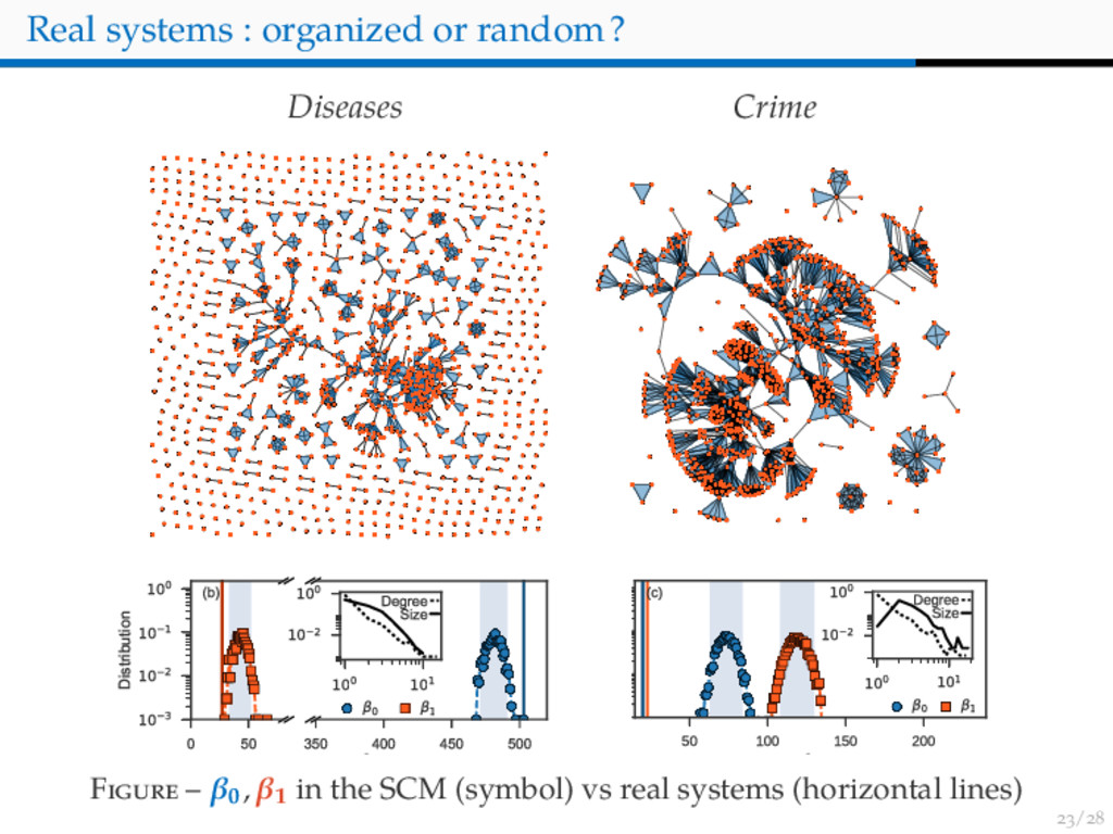
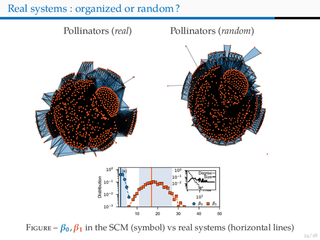
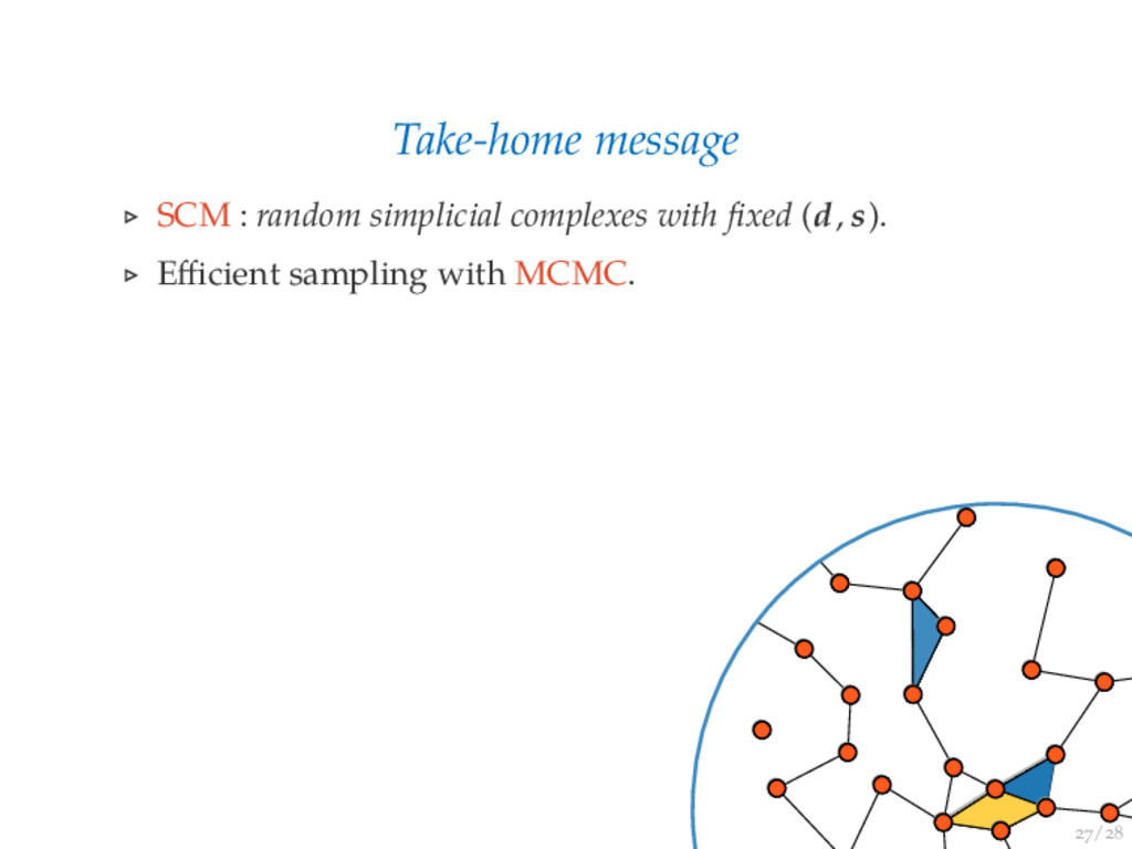
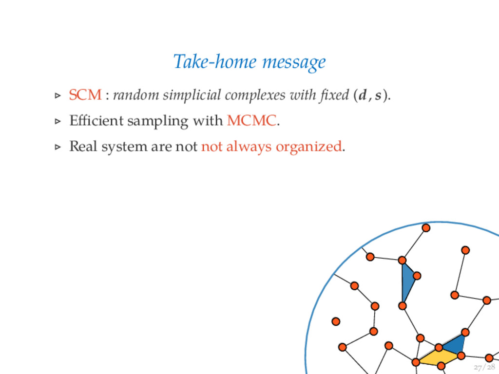
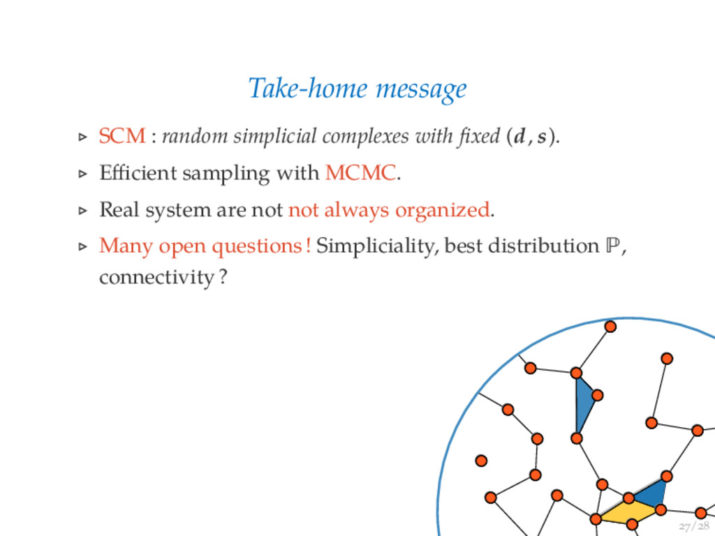
Simplicial complexes are now a popular alternative to networks when it comes to describing the structure of complex systems, primarily because they encode multi-node interactions explicitly. With this new description comes the need for principled null models that allow for easy comparison with empirical data. We propose a natural candidate, the simplicial configuration model. The core of our contribution is an efficient and uniform Markov chain Monte Carlo sampler for this model. We demonstrate its usefulness in a short case study by investigating the topology of three real systems and their randomized counterparts (using their Betti numbers). For two out of three systems, the model allows us to reject the hypothesis that there is no organization beyond the local scale.

Transcript

1. HONS
   C
   J.-G. Young , G. Petri , F. Vaccarino , , A. Patania ,
   June rd,
   Département de physique, de génie physique, et d’optique, Université Laval, Québec, Canada
   ISI Foundation, Turin, Italy
   Dipartimento di Scienze Matematiche, Politecnico di Torino, Torino, Italy
   

   View Slide

2. /
   There are multi-agent interactions
   in complex systems
   Simplicial complexes track this explicitly
   

   View Slide

3. /
   Why simplicial complexes?
   No loss of information upon projection
   

   View Slide

4. /
   Why simplicial complexes?
   No loss of information upon projection
   

   View Slide

5. /
   Why simplicial complexes?
   Efficient compression of the structure
   

   View Slide

6. /
   Why simplicial complexes?
   Efficient compression of the structure
   

   View Slide

7. /
   Disease regulation dataset
   (facets : genes, nodes : human diseases)
   [Goh et al., PNAS, , ( )]
   Diseasome - facets column 1
   

   View Slide

8. /
   Problem we address :
   How to assess the significance
   of the properties of simplicial complexes?
   

   View Slide

9. /
   Outline
   Simplicial complexes and null models
   Simplicial configuration model
   The sampling problem and its solution
   

   View Slide

10. /
    Outline
    Simplicial complexes and null models
    Simplicial configuration model
    The sampling problem and its solution
    The shape of real complex systems : random or organized?
    Homology and Betti numbers
    

    View Slide

11. T
    /
    

    View Slide

12. /
    The simplicial configuration model : basic definitions
    2
    3
    4
    5
    1
    F
    Degree sequence : d (2, 2, 1, 2, 1)
    Size sequence : s (3, 3, 2)
    

    View Slide

13. /
    The simplicial configuration model : basic definitions
    2
    3
    4
    5
    1
    F
    Degree sequence : d (2, 2, 1, 2, 1)
    Size sequence : s (3, 3, 2)
    

    View Slide

14. /
    The simplicial configuration model : basic definitions
    2
    3
    4
    5
    1
    F
    Degree sequence : d (2, 2, 1, 2, 1)
    Size sequence : s (3, 3, 2)
    

    View Slide

15. /
    The simplicial configuration model : the ensemble
    The Simplicial Configuration Model (SCM) is the distribution :
    Pr(K; d, s) 1/|Ω(d, s)|
    Ω(d, s) : number of simplicial complexes with sequences (d, s)
    2
    3
    4
    5
    1
    Generalizes [Courtney and Bianconi, Phys. Rev. E , ( )]
    

    View Slide

16. /
    The simplicial configuration model : the ensemble
    The Simplicial Configuration Model (SCM) is the distribution :
    Pr(K; d, s) 1/|Ω(d, s)|
    Ω(d, s) : number of simplicial complexes with sequences (d, s)
    Generalizes [Courtney and Bianconi, Phys. Rev. E , ( )]
    

    View Slide

17. S SCM
    /
    

    View Slide

18. /
    Sampling : Change of representation
    2
    3
    4
    5
    1
    S : B
    Factor graph ensemble with degree sequences (d, s) ...
    

    View Slide

19. /
    Sampling : Change of representation
    2
    3
    4
    5
    1
    S : B
    Factor graph ensemble with degree sequences (d, s) ...
    

    View Slide

20. /
    Sampling : Change of representation
    2
    3
    4
    5
    1
    S : B
    Factor graph ensemble with degree sequences (d, s) ...
    ... and two additional constraints (mapping bijective)
    ◦ No
    ◦ No
    

    View Slide

21. /
    Sampling : Constraints
    Input sequences : (d, s) ([2, 2, 1, 2, 1], [3, 3, 2])
    Correct mapping
    2
    3
    4
    5
    1
    2
    3
    4
    5
    1
    Bipartite graph Simplicial complex
    Output sequences : (d, s) ([2, 2, 1, 2, 1], [3, 3, 2])
    

    View Slide

22. /
    Sampling : Constraints
    Input sequences : (d, s) ([2, 2, 1, 2, 1], [3, 3, 2])
    Constraint not respected : No multiedges
    2
    3
    4
    5
    1
    2
    3
    4
    5
    1
    Bipartite graph Simplicial complex
    Output sequences : (d, s) ([1, 2, 1, 1, 1], [2, 2, 2])
    

    View Slide

23. /
    Sampling : Constraints
    Input sequences : (d, s) ([2, 2, 1, 2, 1], [3, 3, 2])
    Constraint not respected : No included neighborhoods
    2
    3
    4
    5
    1
    2
    3
    4
    5
    1
    Bipartite graph Simplicial complex
    Output sequences : (d, s) ([1, 1, 1, 1, 1], [3, 0, 2])
    

    View Slide

24. /
    Consequence :
    Uniform distribution over bipartite graphs
    Uniform distribution over simplicial complexes
    

    View Slide

25. /
    Consequence :
    Uniform distribution over bipartite graphs
    Uniform distribution over simplicial complexes
    

    View Slide

26. /
    Sampling : Possible sampling strategies
    

    View Slide

27. /
    Sampling : Possible sampling strategies
    Rejection sampling (stub matching + rejection)
    All bipartite graphs with
    sequences (d,s)
    No constraints violated
    Reject
    

    View Slide

28. /
    Sampling : Possible sampling strategies
    Rejection sampling (stub matching + rejection)
    P : Far too many rejections! Loose upper bound :
    Pr[reject] > exp −1
    2
    d2 / d − 1 s2 / s − 1
    All bipartite graphs with
    sequences (d,s)
    Reject
    

    View Slide

29. /
    Sampling : Possible sampling strategies
    Rejection sampling (stub matching + rejection)
    P : Far too many rejections! Loose upper bound :
    Pr[reject] > exp −1
    2
    d2 / d − 1 s2 / s − 1
    Markov Chain Monte Carlo The natural choice!
    

    View Slide

30. 2
    3
    4
    5
    1
    2
    3
    4
    5
    1
    2
    3
    4
    5
    1
    2
    3
    4
    5
    1
    2
    3
    4
    5
    1
    2
    3
    4
    5
    1
    2
    3
    4
    5
    1
    4
    2
    3
    4
    5
    1
    2
    3
    4
    5
    1
    2
    3
    4
    5
    1
    2
    3
    4
    5
    1
    2
    3
    4
    5
    1
    2
    3
    4
    5
    1
    2
    3
    4
    5
    1
    MCMC
    

    View Slide

31. View Slide

32. View Slide

33. View Slide

34. /
    Sampling : MCMC Details
    M
    Pick L ∼ P random edges in bipartite graph
    P can be , we use Pr[L ] exp[λ ]/Z
    Rewire edges. If multiedge or included neighbors, reject.
    Similar to [Miklós–Erdős–Soukup, Electron. J. Combin., , ( )]
    2
    3
    4
    5
    1
    2
    3
    4
    5
    1
    2
    3
    4
    5
    1
    2
    3
    4
    5
    1
    2
    3
    4
    5
    1
    

    View Slide

35. /
    Sampling : MCMC Details
    M
    Pick L ∼ P random edges in bipartite graph
    P can be , we use Pr[L ] exp[λ ]/Z
    Rewire edges. If multiedge or included neighbors, reject.
    Similar to [Miklós–Erdős–Soukup, Electron. J. Combin., , ( )]
    MCMC is uniform over Ω(d, s)
    Move set yields aperiodic chain
    ∗
    Move set connects the space
    100 101 102 103 104
    Lmax
    0
    2500
    5000
    7500
    Edit distance
    = 0
    = 1
    = +1
    (a)
    

    View Slide

36. T :
    ?
    /
    

    View Slide

37. /
    SCM has a null model : concept
    N :
    Is the quantity f (X) close to f (K) for random simplicial
    complexes X ∼ SCM[d(K), s(K)]?
    

    View Slide

38. /
    SCM has a null model : concept
    N :
    Is the quantity f (X) close to f (K) for random simplicial
    complexes X ∼ SCM[d(K), s(K)]?
    50 100 150 200
    10 3
    10 2
    10 1
    100
    Distribution
    Property
    I Pr[| f (K) − f (X)| < ] ≈ 1
    Yes : K is typical, the local quantities d, s explain f.
    

    View Slide

39. /
    SCM has a null model : concept
    N :
    Is the quantity f (X) close to f (K) for random simplicial
    complexes X ∼ SCM[d(K), s(K)]?
    50 100 150 200
    10 3
    10 2
    10 1
    100
    Distribution
    Property
    I Pr[| f (K) − f (X)| < ] 1
    No : K is atypical, K is organized beyond the local scale.
    

    View Slide

40. /
    So ... are real systems organized?
    

    View Slide

41. /
    Disease regulation dataset (true system)
    (facets : genes, nodes : human diseases)
    [Goh et al., PNAS, , ( )]
    Diseasome - facets column 1
    

    View Slide

42. /
    Disease regulation dataset (random instance)
    (facets : genes, nodes : human diseases)
    [Goh et al., PNAS, , ( )]
    Diseasome - SCM (facets column 1)
    

    View Slide

43. /
    Crimes in St-Louis (true system)
    (facets : people, nodes : crimes)
    [Rosenfeld et al., ( )]
    Moreno crime - facets column 1
    

    View Slide

44. /
    Crimes in St-Louis (random instance)
    (facets : people, nodes : crimes)
    [Rosenfeld et al., ( )]
    Moreno crime - SCM (facets column 1)
    

    View Slide

45. /
    So ... are real systems random?
    

    View Slide

46. /
    So ... are real systems random?
    Visibly not.
    

    View Slide

47. /
    How to quantify this : Homology in seconds
    2
    3
    4
    5
    1
    2
    3
    4
    5
    1
    Q
    Done with homology.
    Results summarized with B β
    0,β
    1,...
    βk : counts the number of dimension k holes
    

    View Slide

48. /
    Real systems : organized or random?
    Diseases Crime
    Diseasome - facets column 1 Moreno crime - facets column 1
    0 50
    10 3
    10 2
    10 1
    100
    Distribution
    350 400 450 500
    k
    1
    0
    100 101
    10 2
    100
    Degree
    Size
    (b)
    50 100 150 200
    k
    10 3
    10 2
    10 1
    100
    Distribution
    0 1
    100 101
    10 2
    100
    Degree
    Size
    (c)
    F – β0
    , β1 in the SCM (symbol) vs real systems (horizontal lines)
    

    View Slide

49. /
    Real systems : organized or random?
    Pollinators (real) Pollinators (random)
    Pollonators - facets column 0
    Pollinators - SCM (facets column 0)
    10 20 30 40 50
    k
    10 3
    10 2
    10 1
    100
    Distribution
    0 1
    101
    10 2
    10 1
    100
    Degree
    Size
    (a)
    F – β0
    , β1 in the SCM (symbol) vs real systems (horizontal lines)
    

    View Slide

50. /
    Software and tutorials : github.com/jg-you/scm
    

    View Slide

51. /
    Software and tutorials : github.com/jg-you/scm
    

    View Slide

52. /
    Software and tutorials : github.com/jg-you/scm
    

    View Slide

53. /
    Selected references
    O
    ( ) J.-G. Young, G. Petri, F. Vaccarino and A. Patania,
    arxiv : . ( )
    Equilibrium random ensembles
    ( ) O. Courtney and G. Bianconi, Phys. Rev. E , ( )
    ( ) K. Zuev, O. Eisenberg and K. Krioukov, J. Phys. A , ( )
    Sampling
    ( ) B. K. Fosdick, et al., arXiv : . ( )
    

    View Slide

54. /
    Take-home message
    SCM : random simplicial complexes with fixed (d, s).
    

    View Slide

55. /
    Take-home message
    SCM : random simplicial complexes with fixed (d, s).
    Efficient sampling with MCMC.
    

    View Slide

56. /
    Take-home message
    SCM : random simplicial complexes with fixed (d, s).
    Efficient sampling with MCMC.
    Real system are not not always organized.
    

    View Slide

57. /
    Take-home message
    SCM : random simplicial complexes with fixed (d, s).
    Efficient sampling with MCMC.
    Real system are not not always organized.
    Many open questions! Simpliciality, best distribution P,
    connectivity?
    

    View Slide

58. /
    Take-home message
    SCM : random simplicial complexes with fixed (d, s).
    Efficient sampling with MCMC.
    Real system are not not always organized.
    Many open questions! Simpliciality, best distribution P,
    connectivity?
    Reference : arxiv.org/1705.10298
    Software : github.com/jg-you/scm
    

    View Slide

59. /
    Reference : arxiv.org/1705.10298
    Software : github.com/jg-you/scm
    info@jgyoung.ca jgyoung.ca @_jgyou
    

    View Slide