Spectral clustering of graphs

2016 CRM Summer School on Spectral Theory:Spectral Theory and Applications

Transcript

1. S CRM S S S T A J.-G. Young July , Département de physique, de génie physique, et d’optique Université Laval, Québec, Canada
8. Content . Motivations . Bisection : the spectral method . General case : graph clustering . Two experiments . Conclusion
9. M
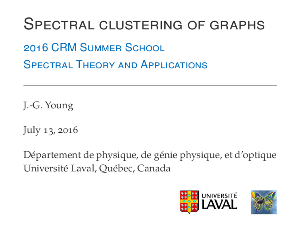
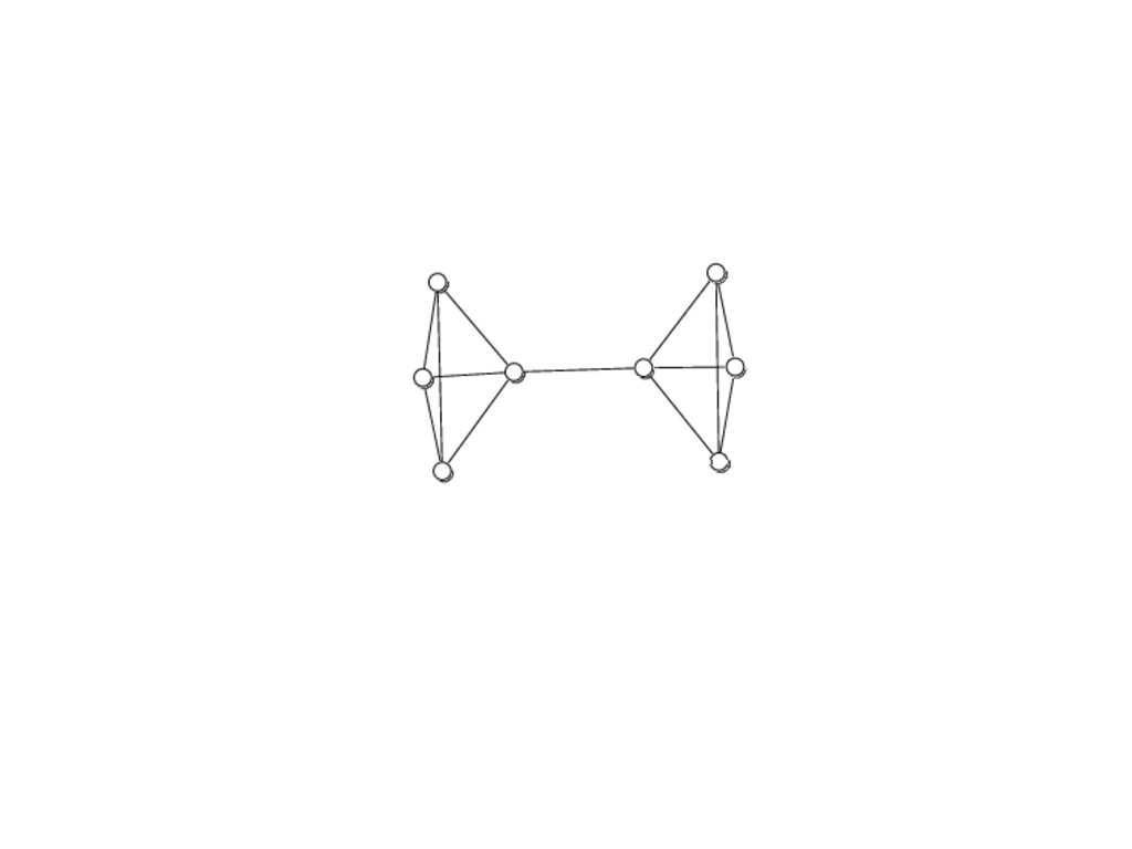
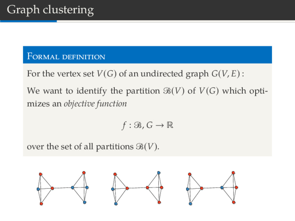
10. Graph clustering F For the vertex set V(G) of an undirected graph G(V, E) : We want to identify the partition B(V) of V(G) which opti- mizes an objective function f : B, G → R over the set of all partitions B(V).
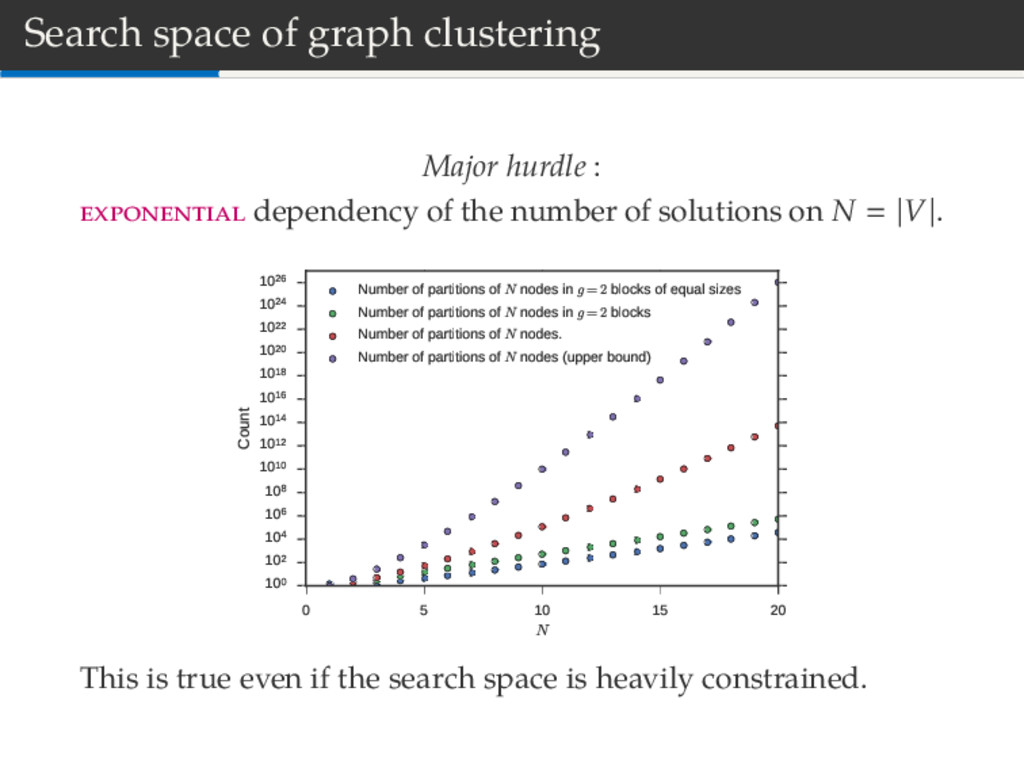
11. Search space of graph clustering Major hurdle : dependency of the number of solutions on N |V|. 0 5 10 15 20 N 100 102 104 106 108 1010 1012 1014 1016 1018 1020 1022 1024 1026 Count Number of partitions of N nodes in g=2 blocks of equal sizes Number of partitions of N nodes in g=2 blocks Number of partitions of N nodes. Number of partitions of N nodes (upper bound) This is true even if the search space is heavily constrained.
12. Hardness of clustering ( ) NP-H P : Problems solvable in polynomial time (easy) NP : Problems solvable in non-deterministic polynomial time (hard) NP-C : Equivalence class of NP (hard) NP-H : Problems which are at least as hard as the hardest problem in NP-C (hardest)
13. B :
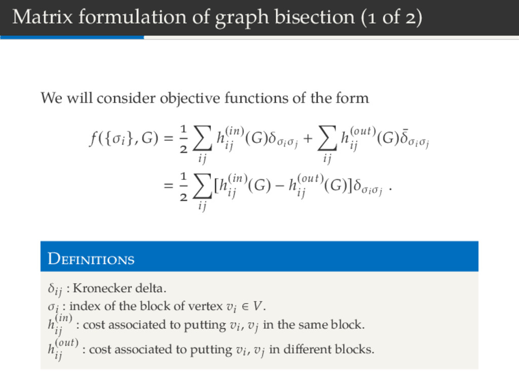
14. Matrix formulation of graph bisection ( of ) We will consider objective functions of the form f ({σi }, G) ij h(in) ij (G)δσi σj + ij h(out) ij (G) ¯ δσi σj ij [h(in) ij (G) − h(out) ij (G)]δσi σj . D δij : Kronecker delta. σi : index of the block of vertex vi ∈ V. h(in) ij : cost associated to putting vi, vj in the same block. h(out) ij : cost associated to putting vi, vj in different blocks.
15. Matrix formulation of graph bisection ( of ) In , either vi ∈ B or vi ∈ B . We denote this with indicator variables si ± . Then si sj      if σi σj − otherwise . and δσi σj ≡ (si sj + )/ .
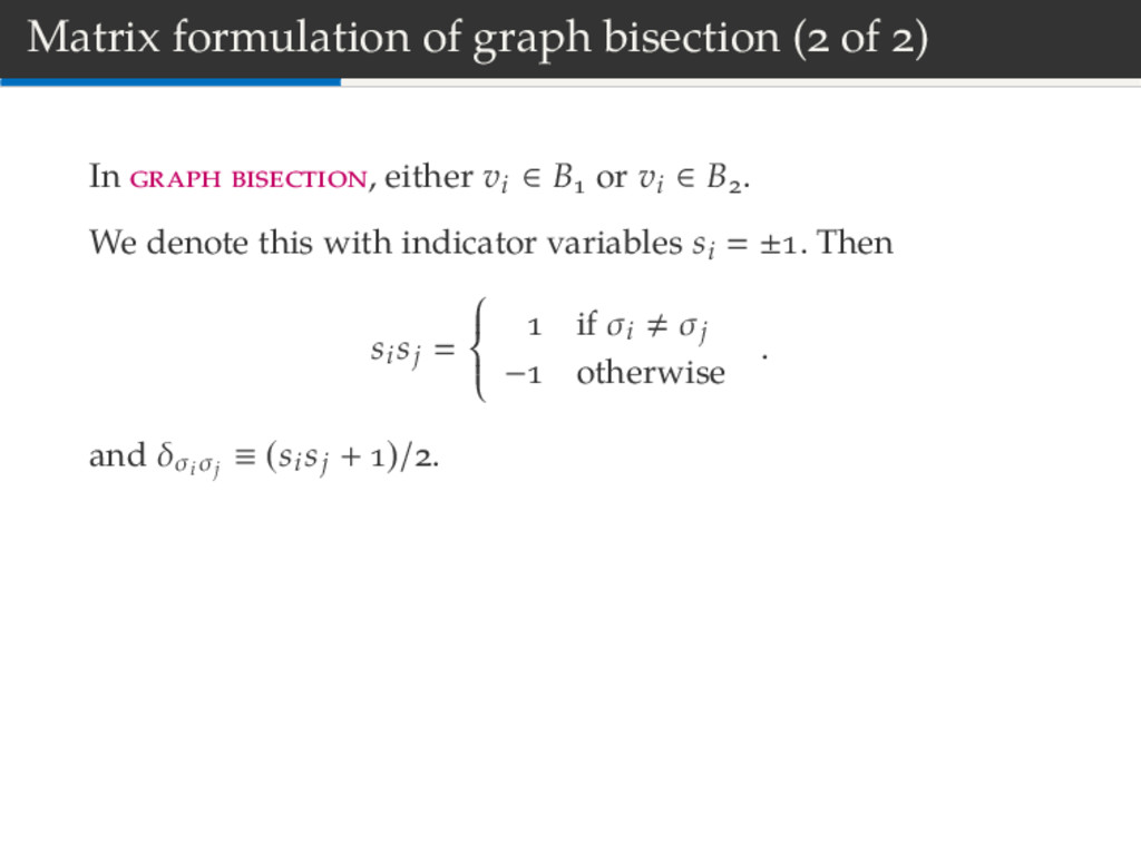
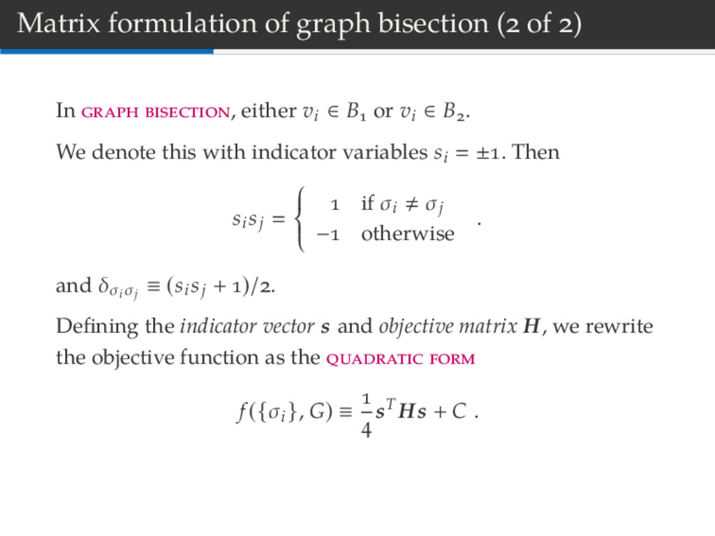
16. Matrix formulation of graph bisection ( of ) In , either vi ∈ B or vi ∈ B . We denote this with indicator variables si ± . Then si sj      if σi σj − otherwise . and δσi σj ≡ (si sj + )/ . Defining the indicator vector s and objective matrix H, we rewrite the objective function as the f ({σi }, G) ≡ sT Hs + C .
17. Example of a objective matrix ( of ) F – Barbell graph B(n , n ) with n , n
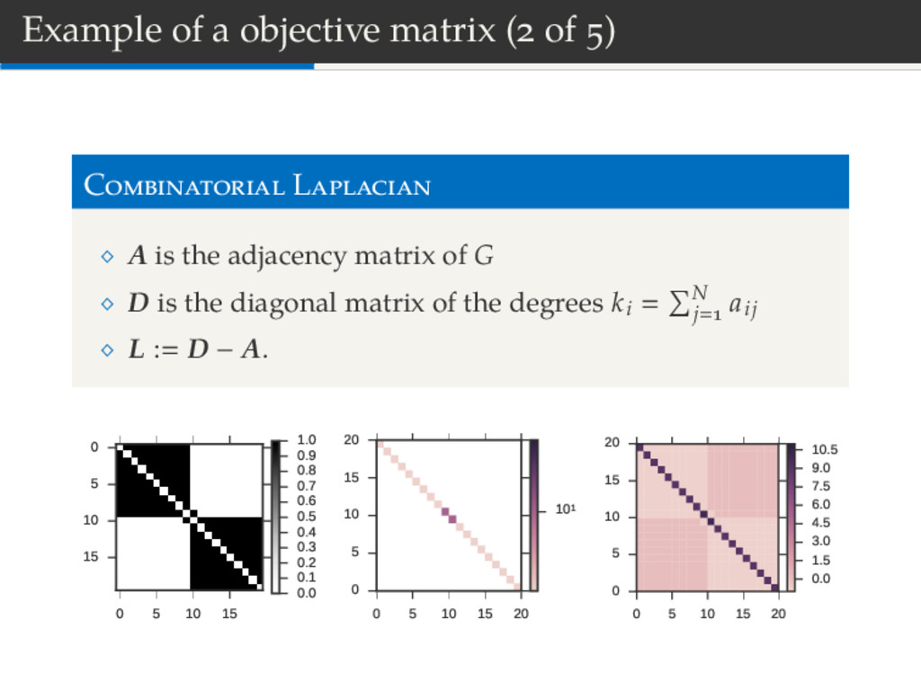
18. Example of a objective matrix ( of ) C L A is the adjacency matrix of G D is the diagonal matrix of the degrees ki N j aij L : D − A. 0 5 10 15 0 5 10 15 0.0 0.1 0.2 0.3 0.4 0.5 0.6 0.7 0.8 0.9 1.0 0 5 10 15 20 0 5 10 15 20 101 0 5 10 15 20 0 5 10 15 20 0.0 1.5 3.0 4.5 6.0 7.5 9.0 10.5
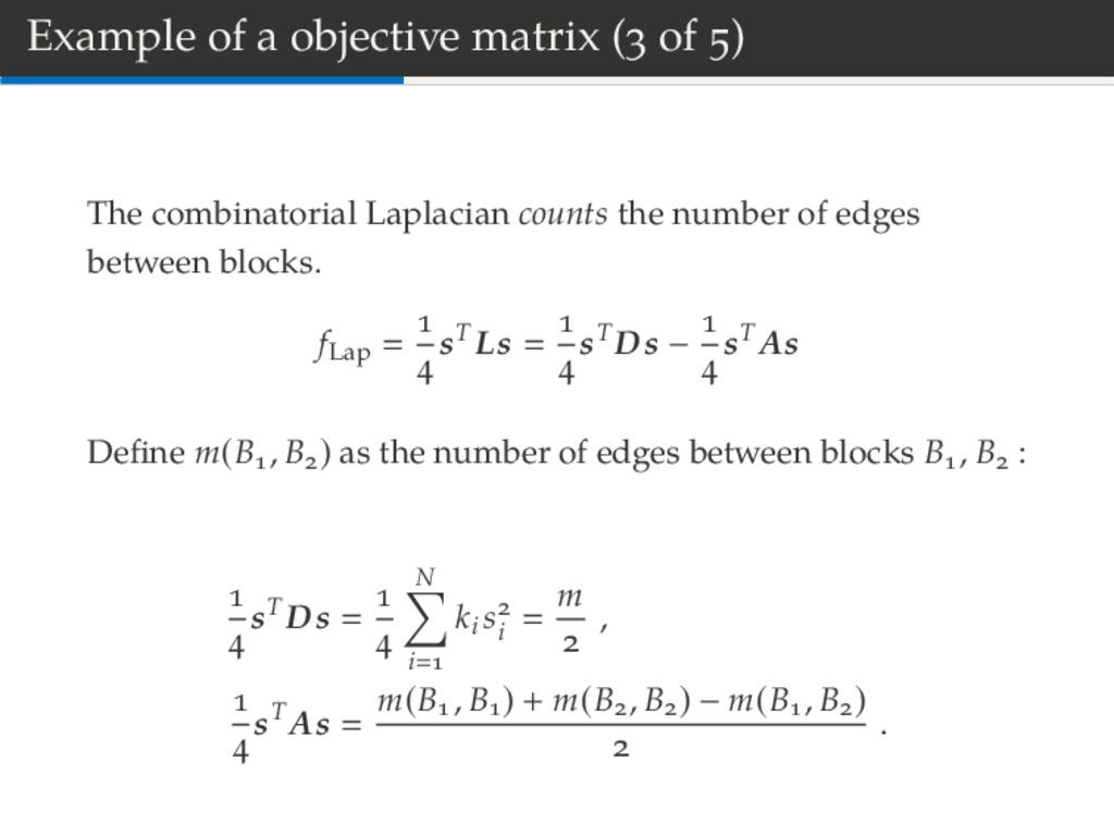
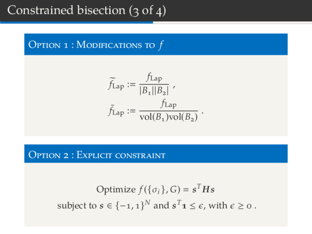
19. Example of a objective matrix ( of ) The combinatorial Laplacian counts the number of edges between blocks. fLap sT Ls sT Ds − sTAs Define m(B , B ) as the number of edges between blocks B , B : sT Ds N i ki s i m , sTAs m(B , B ) + m(B , B ) − m(B , B ) .
20. Example of a objective matrix ( of ) F – Barbell graph B(n , n ) with n , n
21. Example of a objective matrix ( of ) F – Barbell graph B(n , n ) with n , n
22. Example of a objective matrix ( of ) O Adjacency matrix A Normalized Laplacians Lsym D− / LD− / , Lrw D− LD Modularity Q A − A H
23. Constrained bisection ( of ) F – Modified Barbell graph.
24. Constrained bisection ( of ) U Optimize f ({σi }, G) sT Hs subject to s ∈ {− , }N . B partitions are often desirable. Unconstrained bisection does not ask for balance.
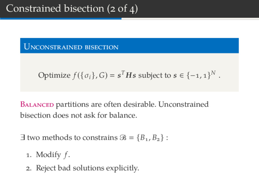
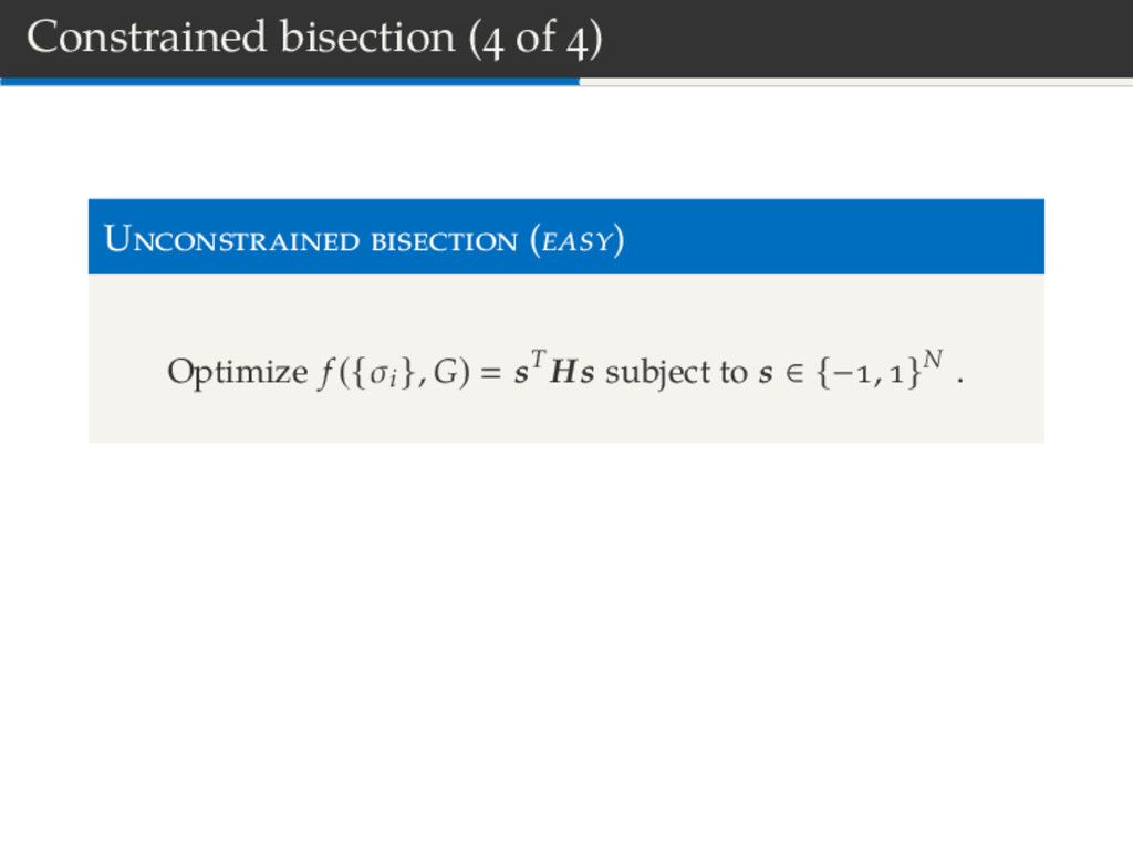
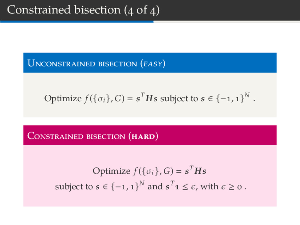
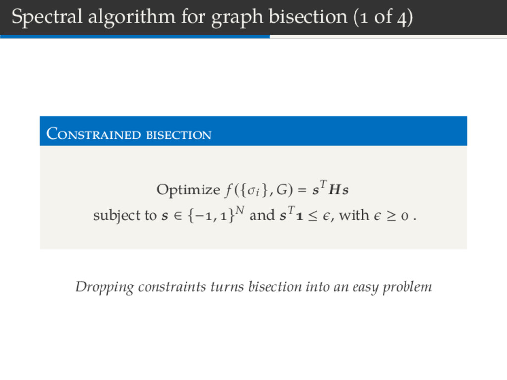
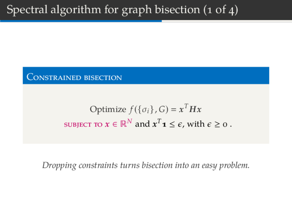
25. Constrained bisection ( of ) U Optimize f ({σi }, G) sT Hs subject to s ∈ {− , }N . B partitions are often desirable. Unconstrained bisection does not ask for balance. ∃ two methods to constrains B {B , B } : . Modify f . . Reject bad solutions explicitly.
26. Constrained bisection ( of ) O : M f fLap : fLap |B ||B | , ¯ fLap : fLap vol(B )vol(B ) . O : E Optimize f ({σi }, G) sT Hs subject to s ∈ {− , }N and sT ≤ , with ≥ .
27. Constrained bisection ( of ) U ( ) Optimize f ({σi }, G) sT Hs subject to s ∈ {− , }N .
28. Constrained bisection ( of ) U ( ) Optimize f ({σi }, G) sT Hs subject to s ∈ {− , }N . C ( ) Optimize f ({σi }, G) sT Hs subject to s ∈ {− , }N and sT ≤ , with ≥ .
29. Spectral algorithm for graph bisection ( of ) C Optimize f ({σi }, G) sT Hs subject to s ∈ {− , }N and sT ≤ , with ≥ . Dropping constraints turns bisection into an easy problem
30. Spectral algorithm for graph bisection ( of ) C Optimize f ({σi }, G) xT Hx x ∈ RN and xT ≤ , with ≥ . Dropping constraints turns bisection into an easy problem.
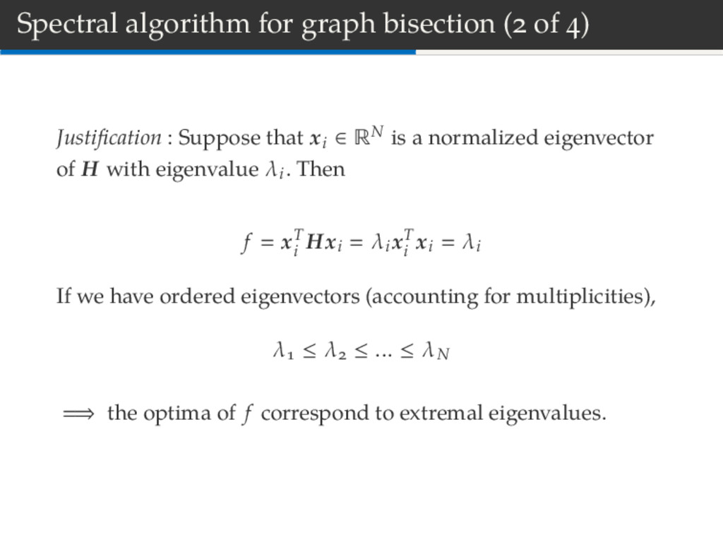
31. Spectral algorithm for graph bisection ( of ) Justification : Suppose that xi ∈ RN is a normalized eigenvector of H with eigenvalue λi. Then f xT i Hxi λi xT i xi λi If we have ordered eigenvectors (accounting for multiplicities), λ ≤ λ ≤ ... ≤ λN ⇒ the optima of f correspond to extremal eigenvalues.
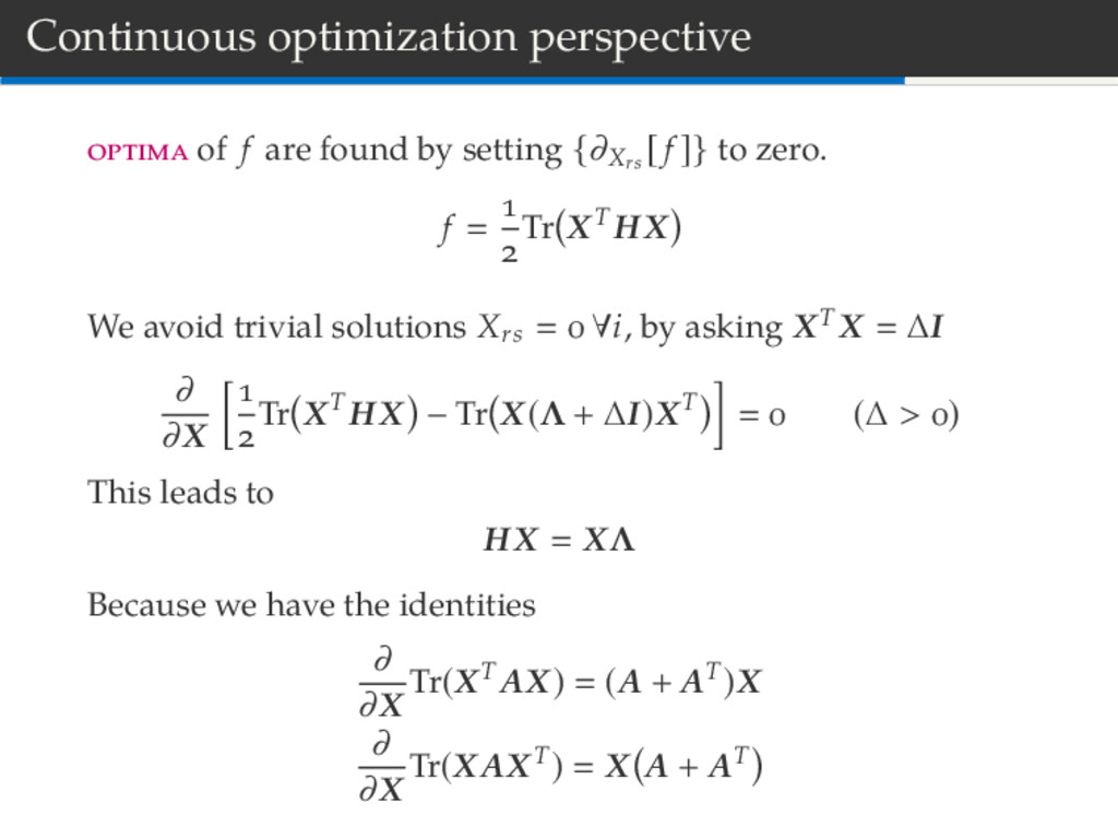
32. Spectral algorithm for graph bisection ( of ) The continuous optimization perspective f xT i Hxi ij hij xi xj of f are found by setting {∂xi [ f ]} to zero. We avoid trivial solutions xi ∀i, by asking i x i ∆, ∆ > ∂ ∂xr        ij hij xi xj − λ i xi − ∆        (∆ > ) Using ∂xr [xi ] δir, we find that j Hij xj λxi ⇔ Hx λx
33. Spectral algorithm for graph bisection ( of ) We have relaxed s → x. How do we recover s ?
34. Spectral algorithm for graph bisection ( of ) We have relaxed s → x. How do we recover s ? In the , we can show that the sign of xi ∈ x is a good predictor of the nearest s.
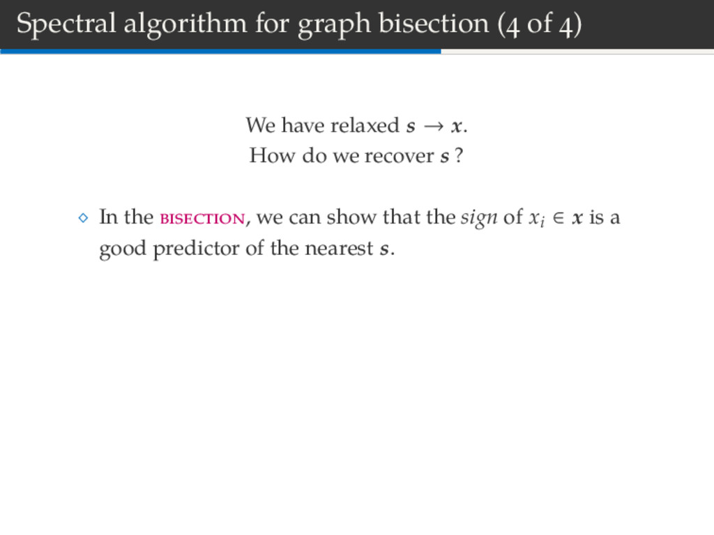
35. Spectral algorithm for graph bisection ( of ) We have relaxed s → x. How do we recover s ? In the , we can show that the sign of xi ∈ x is a good predictor of the nearest s. In general, we can use K-Means to minimize argminB K r i∈Br ||xi − µr || I : Reject solutions that do not satisfy xT ≤ .
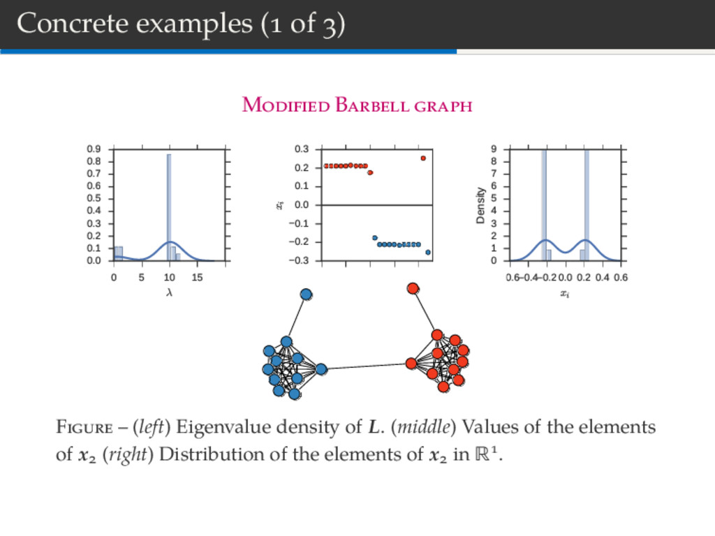
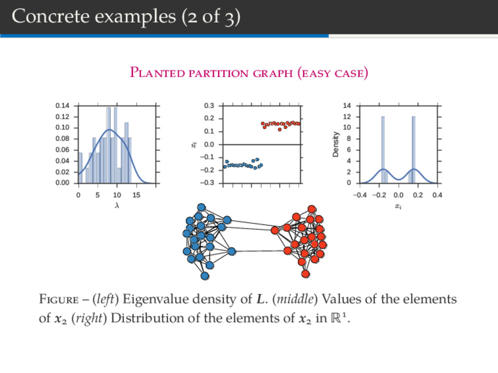
36. Concrete examples ( of ) M B 0 5 10 15 20 λ 0.0 0.1 0.2 0.3 0.4 0.5 0.6 0.7 0.8 0.9 0 5 10 15 20 i 0.3 0.2 0.1 0.0 0.1 0.2 0.3 xi 0.6 0.4 0.20.0 0.2 0.4 0.6 xi 0 1 2 3 4 5 6 7 8 9 Density F – (left) Eigenvalue density of L. (middle) Values of the elements of x (right) Distribution of the elements of x in R .
37. Concrete examples ( of ) P ( ) 0 5 10 15 20 λ 0.00 0.02 0.04 0.06 0.08 0.10 0.12 0.14 0 5 10 15 20 25 30 35 40 i 0.3 0.2 0.1 0.0 0.1 0.2 0.3 xi 0.4 0.2 0.0 0.2 0.4 xi 0 2 4 6 8 10 12 14 Density F – (left) Eigenvalue density of L. (middle) Values of the elements of x (right) Distribution of the elements of x in R .
38. Concrete examples ( of ) P ( ) 0 5 10 15 20 25 λ 0.00 0.02 0.04 0.06 0.08 0.10 0.12 0 5 10 15 20 25 30 35 40 i 0.4 0.2 0.0 0.2 0.4 0.6 xi 0.4 0.2 0.0 0.2 0.4 xi 0.0 0.5 1.0 1.5 2.0 2.5 3.0 3.5 4.0 4.5 Density F – (left) Eigenvalue density of L. (middle) Values of the elements of x (right) Distribution of the elements of x in R .
39. G :
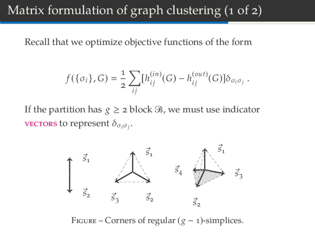
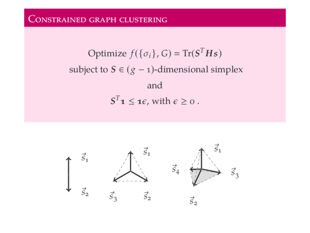
40. Matrix formulation of graph clustering ( of ) Recall that we optimize objective functions of the form f ({σi }, G) ij [h(in) ij (G) − h(out) ij (G)]δσi σj . If the partition has g ≥ block B, we must use indicator to represent δσi σj . s s s s s s s s s F – Corners of regular (g − )-simplices.
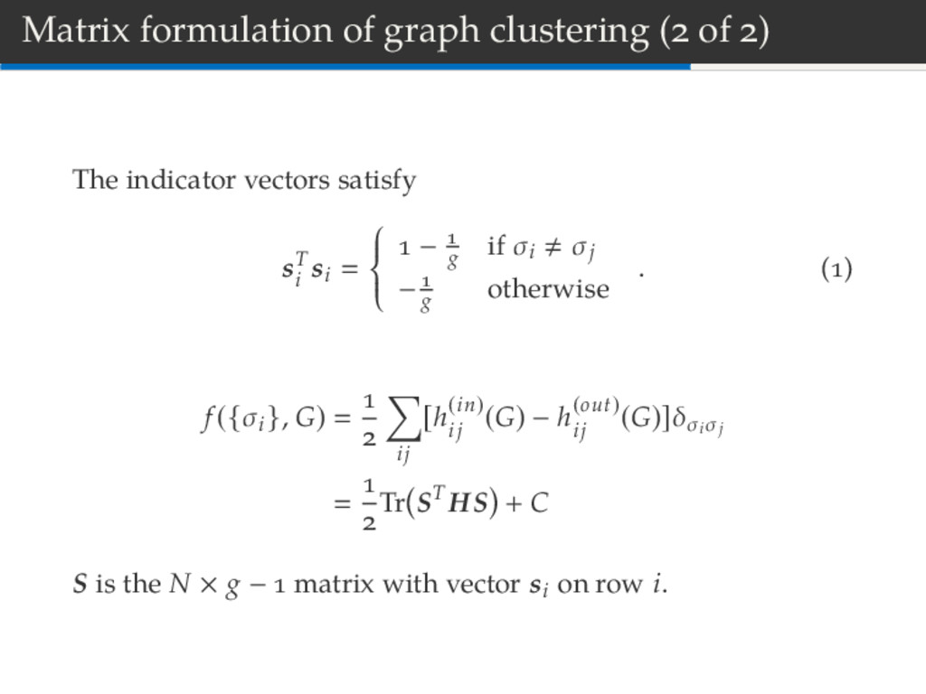
41. Matrix formulation of graph clustering ( of ) The indicator vectors satisfy sT i si      − g if σi σj − g otherwise . ( ) f ({σi }, G) ij [h(in) ij (G) − h(out) ij (G)]δσi σj Tr ST HS + C S is the N × g − matrix with vector si on row i.
42. C Optimize f ({σi }, G) Tr(ST Hs) subject to S ∈ (g − )-dimensional simplex and ST ≤ , with ≥ . s s s s s s s s s
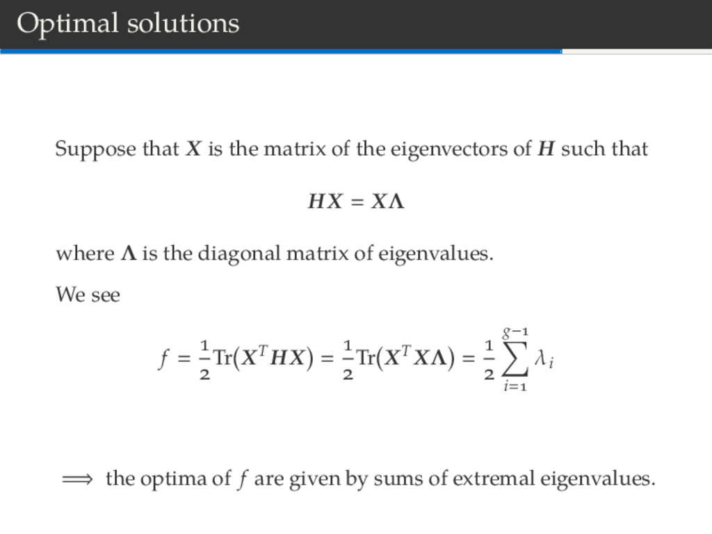
43. Optimal solutions Suppose that X is the matrix of the eigenvectors of H such that HX XΛ where Λ is the diagonal matrix of eigenvalues. We see f Tr XT HX Tr XT XΛ g− i λi ⇒ the optima of f are given by sums of extremal eigenvalues.
44. Continuous optimization perspective of f are found by setting {∂Xrs [ f ]} to zero. f Tr XT HX We avoid trivial solutions Xrs ∀i, by asking XT X ∆I ∂ ∂X Tr XT HX − Tr X(Λ + ∆I)XT (∆ > ) This leads to HX XΛ Because we have the identities ∂ ∂X Tr(XTAX) (A + AT)X ∂ ∂X Tr(XAXT) X A + AT
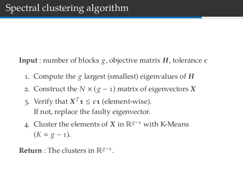
45. Spectral clustering algorithm Input : number of blocks g, objective matrix H, tolerance . Compute the g largest (smallest) eigenvalues of H . Construct the N × (g − ) matrix of eigenvectors X . Verify that XT ≤ (element-wise). If not, replace the faulty eigenvector. . Cluster the elements of X in Rg− with K-Means (K g − ). Return : The clusters in Rg− .
46. Example P ( ) 0 2 4 6 8 10 12 14 16 λ 0.00 0.02 0.04 0.06 0.08 0.10 0.12 0.14 0.3 0.2 0.1 0.0 0.1 0.2 0.3 x(1) i 0.2 0.1 0.0 0.1 0.2 0.3 x(2) i F – (left) Eigenvalue density of L. (right) Elements of x versus the element of x in R .
47. The number of clusters The optimal nb. of blocks is predicted by the ∆i (λi+ − λi ) N 0 5 10 15 20 i 0.00 0.05 0.10 0.15 0.20 (λi+1 − λi)/N Eigengap of C(3,4) 0 5 10 15 20 i 0.00 0.05 0.10 0.15 0.20 (λi+1 − λi)/N Eigengap of C(4,4) 0 5 10 15 20 i 0.00 0.05 0.10 0.15 0.20 (λi+1 − λi)/N Eigengap of C(5,4) 0 5 10 15 20 i 0.00 0.05 0.10 0.15 0.20 (λi+1 − λi)/N Eigengap of C(6,4) F – (left) Caveman graph C( , ) (right) Eigengap of C( , ), , .., .
48. T
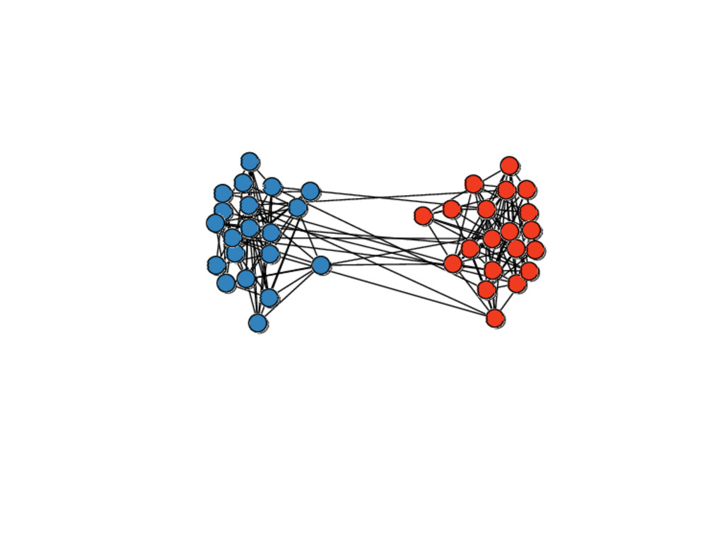
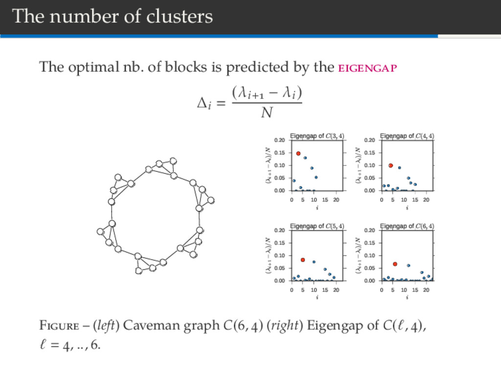
49. Zachary Karate Club 0 2 4 6 8 10 i 0.000 0.005 0.010 0.015 0.020 0.025 0.030 (λi+1 − λi)/N Eigengap of Zachary's Karate Club F – (left) Graph of interactions (right) Statistics of the eigengap [Laplacian matrix].
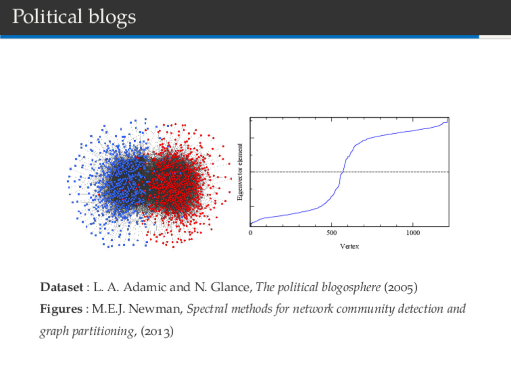
50. Political blogs 0 500 1000 Vertex Eigenvector element Dataset : L. A. Adamic and N. Glance, The political blogosphere ( ) Figures : M.E.J. Newman, Spectral methods for network community detection and graph partitioning, ( )
51. C
52. Take home message Constrained clustering is hard (NP-H ) Relaxing the discrete constraint ⇒ spectral algorithm The spectral approach arises from the continuous optimization perspective The framework is general, arbitrary H.
53. Supplementary Material The slides, lecture notes and python notebook are online at www.jgyoung.ca/crm2016/ Recommended reading E : U. Von Luxburg, A tutorial on spectral clustering, Statistics and computing, ( ), pp. – . C : M. A. Riolo and M. E. J. Newman, First-principles multiway spectral partitioning of graphs, J. Complex Netw., ( ), pp. – .