Quantifying and Controlling for Sources of Technical Variation and Bias in Longitudinal Microbiome Surveys

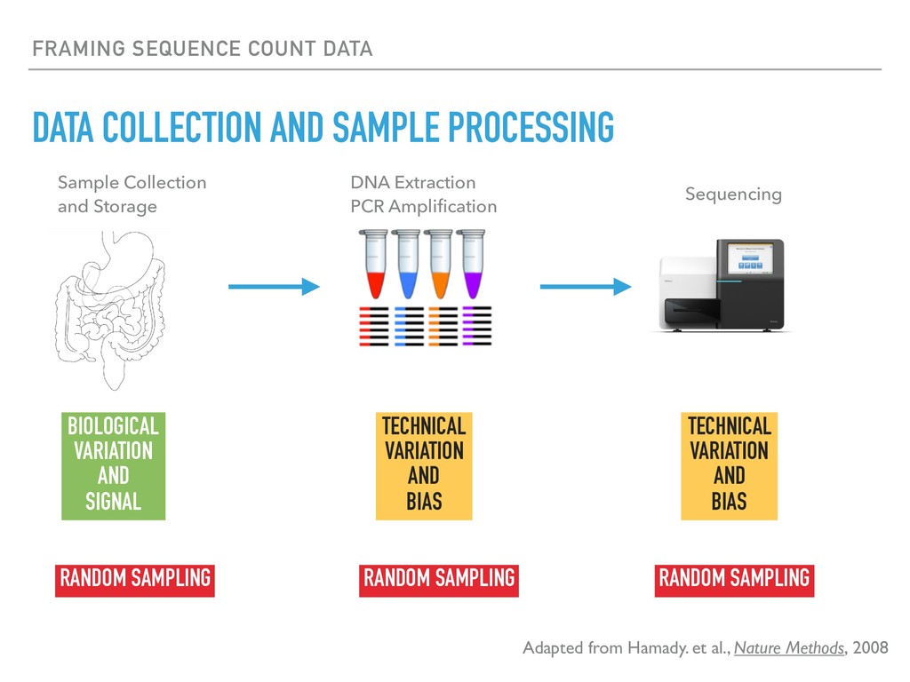
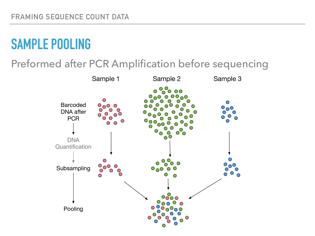
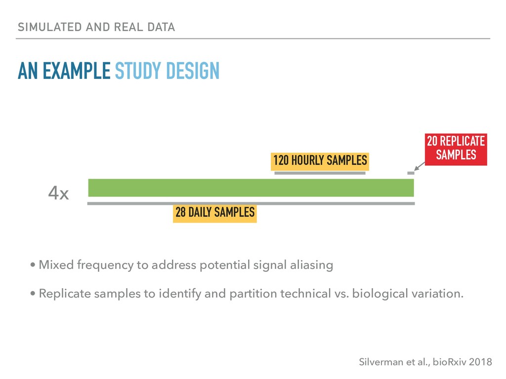
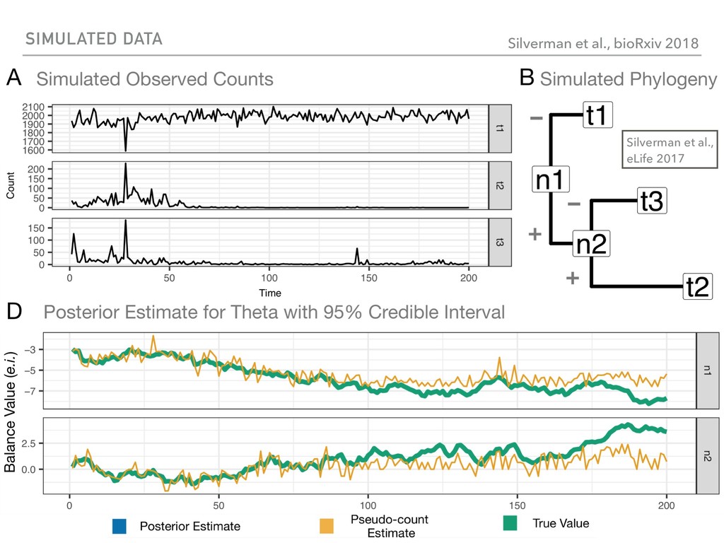
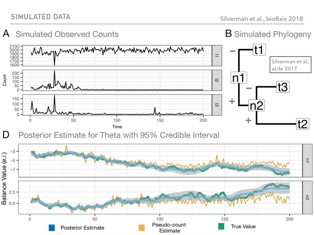
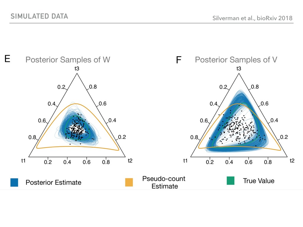
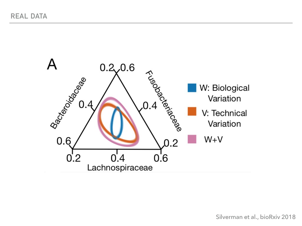
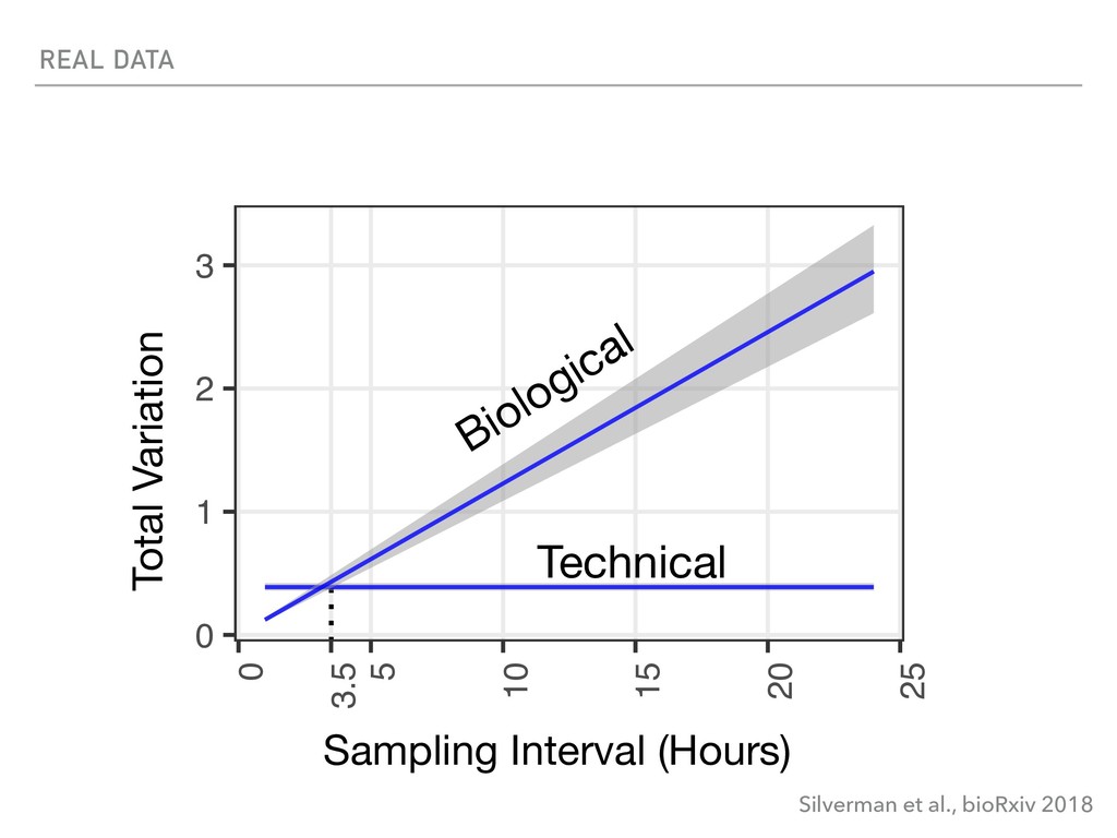
Microbial communities can play important roles in both the health and disease of their hosts. However, measurements of these communities are often confounded by technical variation and bias introduced at a number of stages of sample processing and measurement. Here we develop a flexible class of Bayesian Multinomial-Logistic Normal state space models which explicitly controls for technical variation and bias. Paired with this modeling framework we discuss best practices for experimental design; in particular, the use of technical replicates for quantifying technical variation and calibration curves for measuring bias. We demonstrate our approach through both simulation studies and application to real data.

Transcript

1. TECHNICAL VARIATION AND LONGITUDINAL MICROBIOME DATA JUSTIN D. SILVERMAN MEDICAL SCIENTIST TRAINING PROGRAM COMPUTATIONAL BIOLOGY AND BIOINFORMATICS DUKE UNIVERSITY StatsAtHome.com inschool4life
2. FRAMING CHALLENGES
3. FRAMING SEQUENCE COUNT DATA DATA COLLECTION AND SAMPLE PROCESSING Adapted from Hamady. et al., Nature Methods, 2008 Sample Collection 
 and Storage DNA Extraction
 PCR Amplification Sequencing BIOLOGICAL VARIATION AND SIGNAL TECHNICAL VARIATION AND BIAS TECHNICAL VARIATION AND BIAS RANDOM SAMPLING RANDOM SAMPLING RANDOM SAMPLING
4. FRAMING SEQUENCE COUNT DATA SAMPLE POOLING Preformed after PCR Amplification before sequencing Sample 1 Sample 2 Sample 3 Barcoded DNA after PCR DNA Quantification Subsampling Pooling
5. Group 1 Group 2 Group 3 5 10 15 20 1000 2000 3000 4000 5000 200 400 600 50 100 150 200 250 Time Counts Group 1 Group 2 Group 3 5 10 15 20 100 200 300 400 50 100 25 50 75 100 Time Counts Time Counts A B True Abundance Abundance after Random Sampling FRAMING SEQUENCE COUNT DATA IMPACT OF MULTIVARIATE RANDOM SAMPLING
6. Group 1 Group 2 Group 3 5 10 15 20 1000 2000 3000 4000 5000 200 400 600 50 100 150 200 250 Time Counts Group 1 Group 2 Group 3 5 10 15 20 100 200 300 400 50 100 25 50 75 100 Time Counts Time Counts A B True Abundance Abundance after Random Sampling FRAMING SEQUENCE COUNT DATA IMPACT OF MULTIVARIATE RANDOM SAMPLING NO PROPORTIONS, NOT CLASSICALLY COMPOSITIONAL BUT SAMPLING CAUSES COMPOSITIONAL-LIKE EFFECTS
7. GENERAL MODELING APPROACH
8. CENTRAL THEME MULTINOMIAL-LOGISTIC NORMAL •Handles sampling zeros and ≈ biological zeros •Allows positive and negative covariation between taxa •Models Multiplicative Errors ILR = "Isometric Log-Ratio" Transform
9. TIME-SERIES MODELING
10. BUILDING A FRAMEWORK MODELING TIME-EVOLUTION Silverman et al., bioRxiv 2018 True State with Biological Noise Addition of Technical Noise Observed Counts Priors
11. BUILDING A FRAMEWORK MODELING TIME-EVOLUTION θ0 θ1 θ2 ... θT True State with Biological Noise Silverman et al., bioRxiv 2018 True State with Biological Noise Addition of Technical Noise Observed Counts Priors
12. BUILDING A FRAMEWORK MODELING TIME-EVOLUTION θ0 θ1 θ2 ... θT W1 W2 WT True State with Biological Noise Silverman et al., bioRxiv 2018 True State with Biological Noise Addition of Technical Noise Observed Counts Priors
13. BUILDING A FRAMEWORK MODELING TIME-EVOLUTION η1 η2 ηT θ0 θ1 θ2 ... θT V1 V2 VT W1 W2 WT True State with Biological Noise Addition of Technical Noise Silverman et al., bioRxiv 2018 True State with Biological Noise Addition of Technical Noise Observed Counts Priors
14. BUILDING A FRAMEWORK MODELING TIME-EVOLUTION Y1 Y2 YT η1 η2 ηT θ0 θ1 θ2 ... θT V1 V2 VT W1 W2 WT True State with Biological Noise Observed Counts Addition of Technical Noise Silverman et al., bioRxiv 2018 True State with Biological Noise Addition of Technical Noise Observed Counts Priors
15. BUILDING A FRAMEWORK MODELING TIME-EVOLUTION Y1 Y2 YT η1 η2 ηT θ0 θ1 θ2 ... θT V1 V2 VT W1 W2 WT True State with Biological Noise Observed Counts Addition of Technical Noise ILR Silverman et al., bioRxiv 2018 True State with Biological Noise Addition of Technical Noise Observed Counts Priors
16. BUILDING A FRAMEWORK MODELING TIME-EVOLUTION Define: Inference Goal: Composition with Technical Variation System State Covariance of Technical Variation Covariance of Temporal Evolution ("Biological Variation") Observed Counts and 
 Covariates
17. BUILDING A FRAMEWORK COLLAPSED SAMPLING USING THE KALMAN FILTER Goal:
18. BUILDING A FRAMEWORK COLLAPSED SAMPLING USING THE KALMAN FILTER Goal: Term 2: Using 1st order 
 Markov Structure Arbitrary Prior 1-step ahead predictive
 densities calculable by 
 Kalman filter Product of Multinomial
 densities
19. BUILDING A FRAMEWORK COLLAPSED SAMPLING USING THE KALMAN FILTER Goal: Term 2: Using 1st order 
 Markov Structure Arbitrary Prior 1-step ahead predictive
 densities calculable by 
 Kalman filter Product of Multinomial
 densities Term 1: Can be sampled from directly 
 using Backwards Sampling algorithm
 (aka Kalman Smoother) Θ ⊥ Y | H
20. BUILDING A FRAMEWORK COLLAPSED SAMPLING USING THE KALMAN FILTER Goal: Sampling Algorithm: Step 1: Sample using adaptive HMCMC marginalizing over Θ using Kalman Filter Step 2: Sample using Backwards sampling (aka Kalman Smoother)
21. BUILDING A FRAMEWORK COLLAPSED SAMPLING USING THE KALMAN FILTER Goal: Sampling Algorithm: Step 1: Sample using adaptive HMCMC marginalizing over Θ using Kalman Filter Step 2: Sample using Backwards sampling (aka Kalman Smoother) Summary:
22. BUILDING A FRAMEWORK COLLAPSED SAMPLING USING THE KALMAN FILTER Goal: Sampling Algorithm: Step 1: Sample using adaptive HMCMC marginalizing over Θ using Kalman Filter Step 2: Sample using Backwards sampling (aka Kalman Smoother) Summary: • By inverting the "classic" Metropolis within Gibbs sampler we can take advantage of adaptive Hamiltonian MCMC
23. BUILDING A FRAMEWORK COLLAPSED SAMPLING USING THE KALMAN FILTER Goal: Sampling Algorithm: Step 1: Sample using adaptive HMCMC marginalizing over Θ using Kalman Filter Step 2: Sample using Backwards sampling (aka Kalman Smoother) Summary: • By inverting the "classic" Metropolis within Gibbs sampler we can take advantage of adaptive Hamiltonian MCMC • Θ (typically very high dimensional) can be removed from HMCMC and instead sampled directly using recurrence relationships of Kalman Smoother (very fast)
24. BUILDING A FRAMEWORK Multinomial Logistic-Normal Dynamic Linear Models
25. BUILDING A FRAMEWORK MALLARD Multinomial Logistic-Normal Dynamic Linear Models www.audubon.org
26. PARTITIONING BIOLOGICAL AND TECHNICAL VARIATION
27. SIMULATED AND REAL DATA AN EXAMPLE STUDY DESIGN Silverman et al., bioRxiv 2018 STANDARD LONGITUDINAL MODEL CONDITION TO HANDLE REPLICATES 28 DAILY SAMPLES 120 HOURLY SAMPLES 20 REPLICATE
 SAMPLES 4x • Mixed frequency to address potential signal aliasing • Replicate samples to identify and partition technical vs. biological variation.
28. SIMULATED DATA Silverman et al., bioRxiv 2018 Silverman et al., 
 eLife 2017

29. SIMULATED DATA Silverman et al., bioRxiv 2018 Silverman et al., 
 eLife 2017

30. SIMULATED DATA Silverman et al., bioRxiv 2018
31. REAL DATA Silverman et al., bioRxiv 2018
32. REAL DATA Silverman et al., bioRxiv 2018 0.6 0.2 0.2 0.4 0.6 seq_10 0.2 0.4 0.6 0.8 0.2 8 0 1 2 3 3.5 0 5 10 15 20 25 as.integer(lag) p50 Total Variation Sampling Interval (Hours) Biological Technical B ae Lachnospiraceae W+V
33. OTHER (ACADEMIC) THINGS I LIKE TALKING ABOUT AN APPEAL TO THE COMMUNITY We need more studies that quantify technical variation and bias in a manner that can be used, modeled, and corrected. (Almost) All interesting measurements have error
34. ACKNOWLEDGEMENTS ACKNOWLEDGEMENTS Duke University Lawrence David Sayan Mukherjee Rachael Bloom Heather Durand University de Girona Juan José Egozcue Vera Pawlowsky-Glahn Wife and 
 Collaborator Rachel Silverman Funding Duke Collaborative Quantitative Approaches to Problems in the Basic and Clinical Sciences 
 Duke MSTP NIH T32 xkcd.com StatsAtHome.com inschool4life
35. OTHER (ACADEMIC) THINGS I LIKE TALKING ABOUT SELECTED PROJECTS •Faster Inference for MALLARD Models • Quantifying and removing Batch Variation and Bias using calibration curves and cross-batch standard samples. •There are different types of zero values in sequence count data •Total Relative Augmentation Models (TRAMs) to introduce uncertainty in "total" measurements into compositional models.
36. BUILDING A FRAMEWORK A NOTE ON PRIOR CHOICE All Log-Ratio Transforms: Not so realistic prior: More realistic prior:
37. REAL DATA THINKING IN TERMS OF VARIATION 0.0066 0.0088 0.008 0.0085 0.0067 0.0056 0.015 0.013 0.014 0.011 0.011 0.0081 0.008 0.0062 0.0032 0.026 0.037 0.04 0.041 0.043 0.037 0.031 0.035 0.03 0.028 0.023 0.021 0.048 0.051 0.049 0.04 0.039 0.043 0.038 0.079 0.022 0.035 0.034 0.031 0.031 0.02 0.025 0.061 0.034 0.038 (0.004−0.01) (0.006−0.01) (0.005−0.01) (0.006−0.01) (0.004−0.01)(0.004−0.008) (0.01−0.02) (0.01−0.02) (0.01−0.02) (0.009−0.01) (0.008−0.02) (0.006−0.01) (0.006−0.01)(0.005−0.008) (0.002−0.005) (0.02−0.04) (0.03−0.05) (0.03−0.05) (0.03−0.05) (0.03−0.06) (0.03−0.05) (0.02−0.04) (0.03−0.04) (0.02−0.04) (0.02−0.03) (0.02−0.03) (0.02−0.03) (0.04−0.06) (0.04−0.07) (0.04−0.06) (0.03−0.05) (0.03−0.05) (0.03−0.05) (0.03−0.05) (0.06−0.1) (0.02−0.03) (0.03−0.04) (0.03−0.04) (0.02−0.04) (0.03−0.04) (0.02−0.02) (0.02−0.03) (0.05−0.08) (0.03−0.04) (0.03−0.05) Rikenellaceae Synergistaceae Fusobacteriaceae Enterobacteriaceae Lachnospiraceae Bacteroidaceae Ruminococcaceae Porphyromonadaceae Acidaminococcaceae 0.02 0.04 0.06 p50 Desulfovibrionaceae Acidaminococcaceae Porphyromonadaceae Ruminococcaceae Bacteroidaceae Enterobacteriaceae Fusobacteriaceae Synergistaceae Rikenellaceae Lachnospiraceae Bacteroidaceae 0.0032 (0.0021−0.0048) Median ρ 95% Credible Interval ( ( Lachnospiraceae n.enterobacteriaceae n.oral n.rikenellacae Day 02 Day 09 Day 16 Day 23 Day 30 −2 0 2 4 −8 −4 0 −6 −4 −2 0 2 Balance Value Vessel 1 2 3 4 Posterior 95% credible interval Fusobacteriaceae and Synergistaceae Enterobacteriaceae Rikenellaceae Balance Value (e.i.) B C D Feed Disruption of Vessels 1 and 2 A Silverman et al., bioRxiv 2018
38. REAL DATA THERE ARE SUB-DAILY DYNAMICS A Vessel 3 Vessel 4 Vessel 1 Vessel 2 D ay 21 D ay 22 D ay 23 D ay 24 D ay 25 D ay 21 D ay 22 D ay 23 D ay 24 D ay 25 1.6 2.0 2.4 2.8 1.5 2.0 2.5 3.0 1.50 1.75 2.00 2.25 1.6 2.0 2.4 2.8 Balance Value (e.i.) B Bacteroidetes Proteobacteria Fusobacteria – + Balance Silverman et al., bioRxiv 2018
39. WRAPPING UP CURRENT LIMITATIONS OF MALLARD •Computational Cost ▸ Depends on Assumptions Users are willing to make. ▸ Without simplifying assumptions - 10 bacterial families 700 samples ~ 2 hours. ▸ With simplifying assumptions - 50 families 700 samples ~ 10 minutes ▸ With approximate inference - 100 families 700 samples ~ 1 minute •User Interface