ENAR 2018

Talk in Session on Geometry and Topology in Statistics

Transcript

1. GEOMETRIC METHODS FOR MODELING TIME EVOLUTION OF HUMAN MICROBIOME JUSTIN D. SILVERMAN MEDICAL SCIENTIST TRAINING PROGRAM COMPUTATIONAL BIOLOGY AND BIOINFORMATICS DUKE UNIVERSITY StatsAtHome.com inschool4life
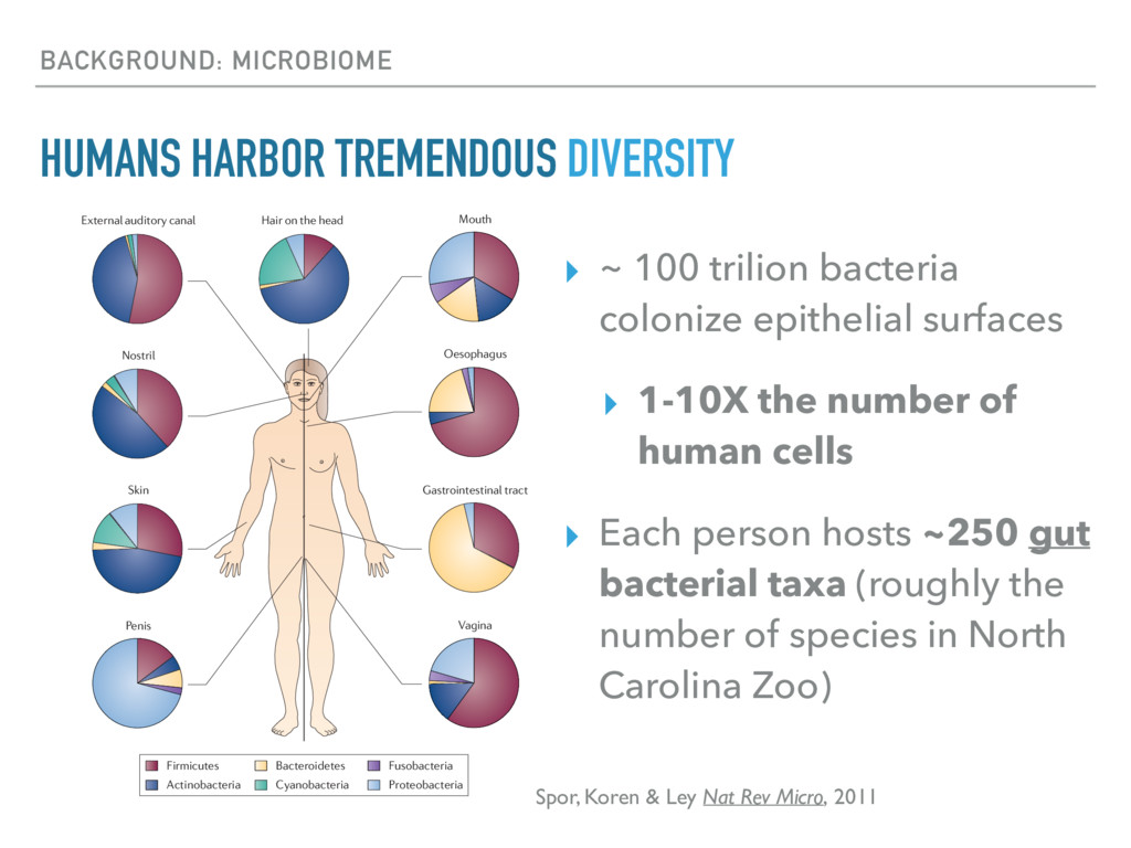
2. BACKGROUND: MICROBIOME HUMANS HARBOR TREMENDOUS DIVERSITY ▸ ~ 100 trilion bacteria colonize epithelial surfaces ▸ 1-10X the number of human cells ▸ Each person hosts ~250 gut bacterial taxa (roughly the number of species in North Carolina Zoo) Nature Reviews | Microbiology External auditory canal Gastrointestinal tract Hair on the head Nostril Skin Firmicutes Actinobacteria Bacteroidetes Cyanobacteria Fusobacteria Proteobacteria Mouth Penis Vagina Oesophagus Variations in those host genes that contribute to proper- ties of the gut habitat therefore have strong potential to affect the variation in the microbiome. Evidence to sup- port a contribution of host genetics to the diversity of the microbial community has been scarce, so the strength of the effect is controversial. However, an increasing number of studies are now evaluating this effect, and the analysis of host genetics is just beginning to be incorpo- rated into studies of how the diversity of the gut bacteria relates to host susceptibility to disease. In this Review, we describe how environmental fac- tors can contribute to variation in the diversity and com- position of the microbiota, and we explore the role of host genes in this process. We also highlight an emerg- ing view of the microbiota: one in which the microbiota itself may be considered as a complex trait that is under host genetic control and that interacts with environmental and host factors in a number of chronic inflammatory diseases. Environmental impact on the microbiota To measure the impact of host genetics on microbial diversity, it is useful to have an understanding of the factors that can influence variation in the microbiota in the absence of host genetic variation, as these environ- mental factors constitute the ‘noise’ that can mask host genetic effects. Model organisms provide a system for controlling variation between identical hosts: genetically inbred animals act as replicate hosts, allowing the impact of environmental factors on the variation in the micro- biota to be assessed. Mice are useful models for studies of human microbial ecology because the intestines of mice harbour communities that are grossly similar in com- position (that is, have similar phylum and family level abundances) to those of human intestines, diverging mainly at the genus level (BOX 1). Husbandry conditions can be standardized across mice, and experiments can Figure 1 | Microbial community composition at different body locations in a healthy human. The relative abundances of the six dominant bacterial phyla in each of the different body sites: the external auditory canal (nine subjects), the hair on the REVIEWS REVIEWS Spor, Koren & Ley Nat Rev Micro, 2011
3. BACKGROUND: MICROBIOME MICROBIOME CAN BE CAUSAL IN DISEASE Turnbaugh et al., Nature 2006 ob/ob +/+ Germ-free mouse increase in body fat (%)
4. FRAMING
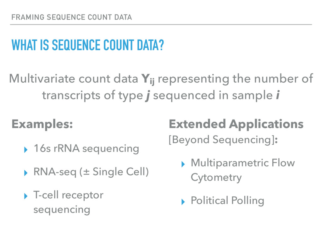
5. Examples: ▸ 16s rRNA sequencing ▸ RNA-seq (± Single Cell) ▸ T-cell receptor sequencing Extended Applications 
 [Beyond Sequencing]: ▸ Multiparametric Flow Cytometry ▸ Political Polling WHAT IS SEQUENCE COUNT DATA? FRAMING SEQUENCE COUNT DATA Multivariate count data Yij representing the number of transcripts of type j sequenced in sample i
6. FRAMING SEQUENCE COUNT DATA DATA COLLECTION AND SAMPLE PROCESSING Adapted from Hamady. et al., Nature Methods, 2008 Sample Collection 
 and Storage DNA Extraction
 PCR Amplification Sequencing Assign Sequences 
 to Samples Denoise Reads
 or Cluster 
 Species 1 Species 2 Species 3 Species 4 Species 5 Species 6 Species 7 Species 8 Species 9 Species 10 Sample 1 23 53 2 44 10 88 94 66 73 67 Sample 2 69 64 70 47 8 97 47 6 64 19 Sample 3 33 100 68 78 59 87 71 31 67 24 Sample 4 5 63 57 27 86 81 83 92 46 62 Sample 5 76 80 46 70 92 92 6 46 37 68 Sample 6 58 7 37 45 25 62 78 44 89 30 Sample 7 10 87 32 80 9 91 59 90 67 77 Sample 8 21 89 73 39 44 80 97 83 80 4 Sample 9 85 77 82 72 15 19 44 4 83 76 Sample 10 67 87 68 58 73 29 87 4 48 79 Sample 11 90 5 28 49 39 20 78 92 12 23 Sample 12 98 93 55 12 54 75 27 95 83 98 Sample 13 31 97 52 9 93 84 45 97 81 27 Sample 14 12 77 22 17 71 12 56 86 18 0 Sample 15 40 30 71 71 54 13 77 96 75 11 Make Count Table
7. FRAMING SEQUENCE COUNT DATA DATA COLLECTION AND SAMPLE PROCESSING Adapted from Hamady. et al., Nature Methods, 2008 Sample Collection 
 and Storage DNA Extraction
 PCR Amplification Sequencing
8. FRAMING SEQUENCE COUNT DATA DATA COLLECTION AND SAMPLE PROCESSING Adapted from Hamady. et al., Nature Methods, 2008 Sample Collection 
 and Storage DNA Extraction
 PCR Amplification Sequencing TECHNICAL VARIATION AND BIAS COUNTING AND BIAS
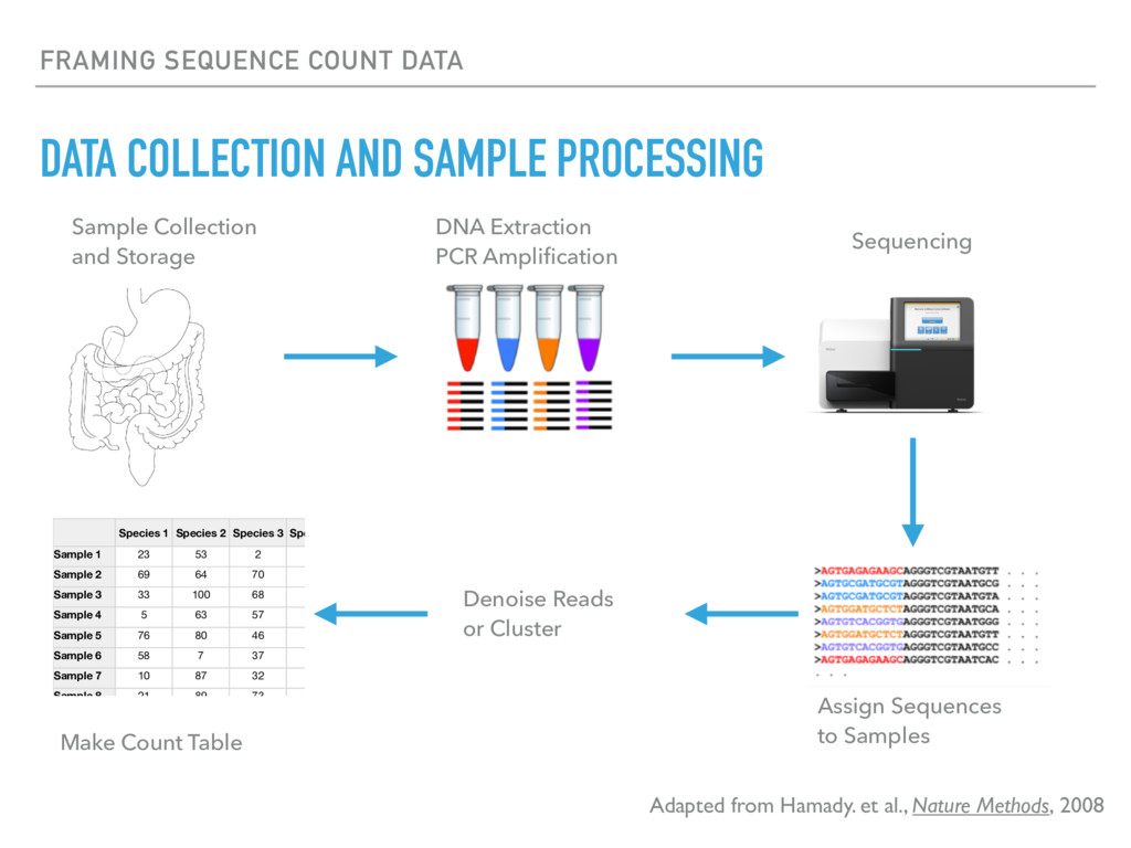
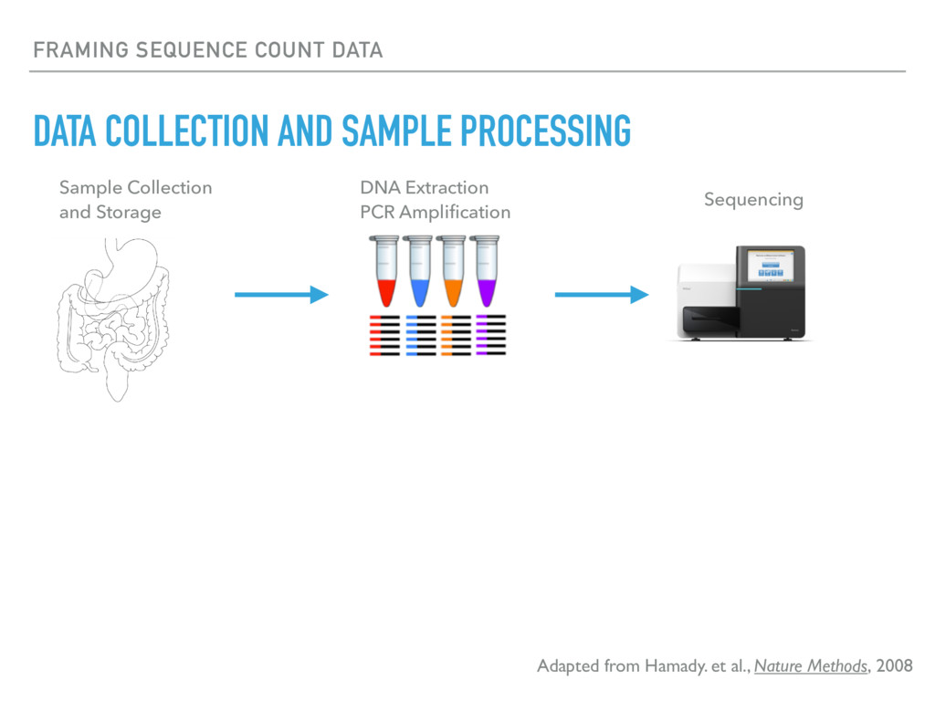
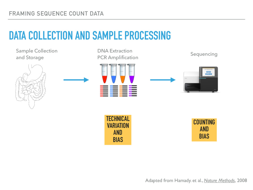
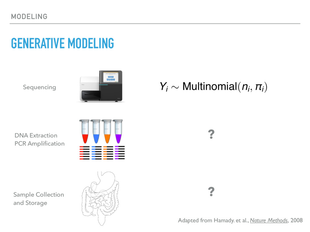
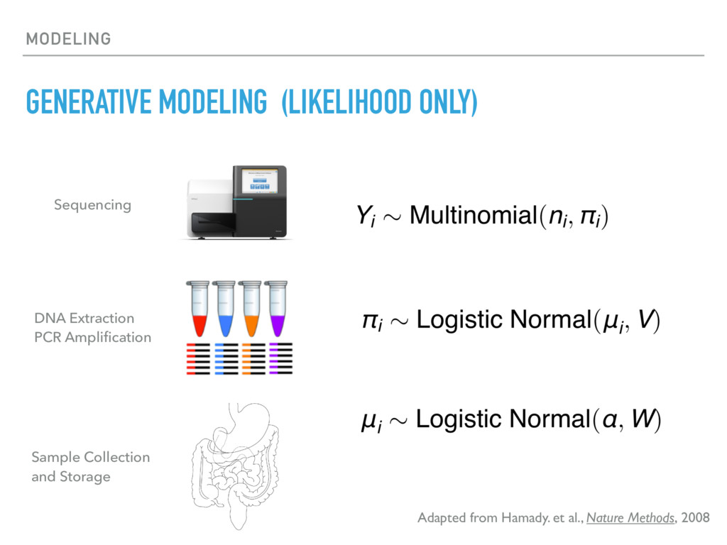
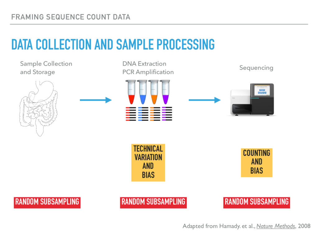
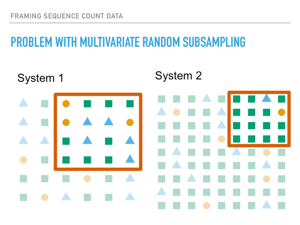
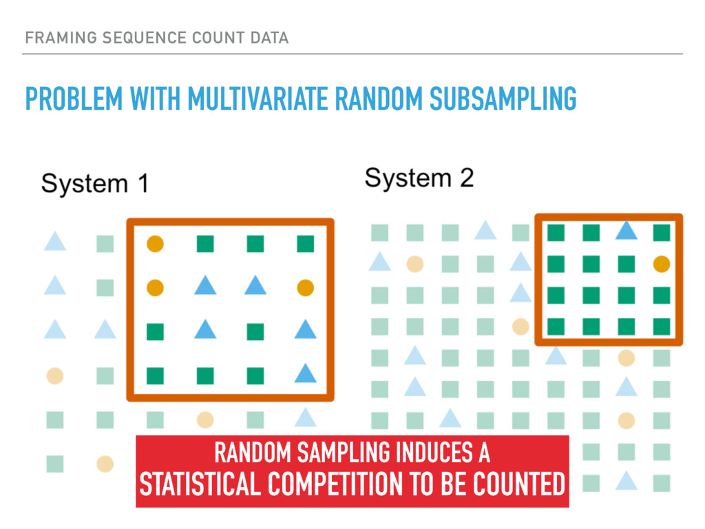
9. FRAMING SEQUENCE COUNT DATA DATA COLLECTION AND SAMPLE PROCESSING Adapted from Hamady. et al., Nature Methods, 2008 Sample Collection 
 and Storage DNA Extraction
 PCR Amplification Sequencing TECHNICAL VARIATION AND BIAS COUNTING AND BIAS RANDOM SUBSAMPLING RANDOM SUBSAMPLING RANDOM SUBSAMPLING
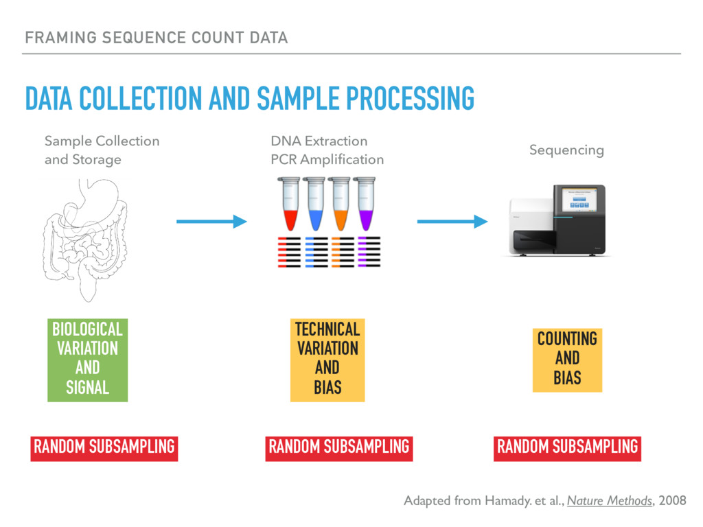
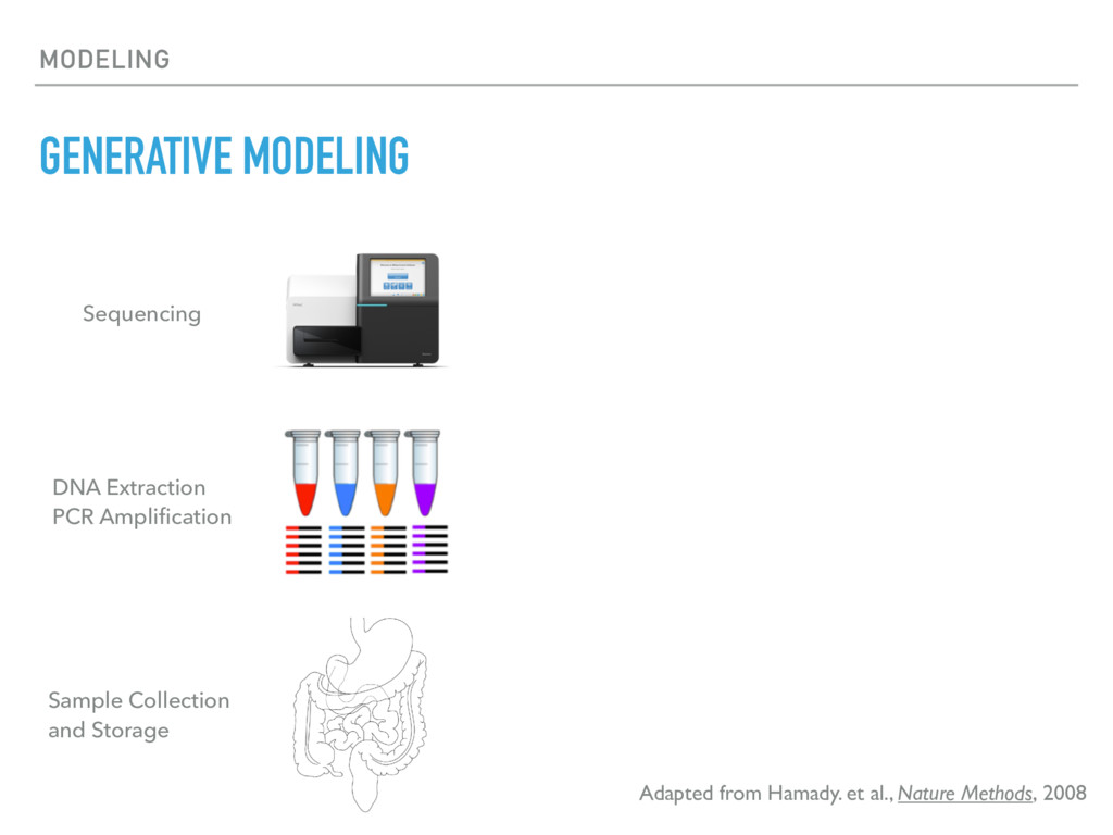
10. FRAMING SEQUENCE COUNT DATA DATA COLLECTION AND SAMPLE PROCESSING Adapted from Hamady. et al., Nature Methods, 2008 Sample Collection 
 and Storage DNA Extraction
 PCR Amplification Sequencing BIOLOGICAL VARIATION AND SIGNAL TECHNICAL VARIATION AND BIAS COUNTING AND BIAS RANDOM SUBSAMPLING RANDOM SUBSAMPLING RANDOM SUBSAMPLING
11. FRAMING SEQUENCE COUNT DATA KEY POINT ▸ Sequencing depth does not correlate with microbial load. ▸ This is purposeful!
12. FRAMING SEQUENCE COUNT DATA PROBLEM WITH MULTIVARIATE RANDOM SUBSAMPLING
13. FRAMING SEQUENCE COUNT DATA PROBLEM WITH MULTIVARIATE RANDOM SUBSAMPLING % Blue % Orange % Green
14. FRAMING SEQUENCE COUNT DATA PROBLEM WITH MULTIVARIATE RANDOM SUBSAMPLING % Blue % Orange % Green
15. FRAMING SEQUENCE COUNT DATA PROBLEM WITH MULTIVARIATE RANDOM SUBSAMPLING % Blue % Orange % Green RANDOM SAMPLING INDUCES A 
 STATISTICAL COMPETITION TO BE COUNTED
16. FRAMING SEQUENCE COUNT DATA THE SPACE OF RELATIVE DATA L B R k k k L+ B+ R=k And all Positive
17. FRAMING SEQUENCE COUNT DATA MICROBIOME DATA IS SPARSE Silverman, et al., eLife 2017
18. MODELING
19. MODELING GENERATIVE MODELING Adapted from Hamady. et al., Nature Methods, 2008 Sample Collection 
 and Storage DNA Extraction
 PCR Amplification Sequencing
20. MODELING GENERATIVE MODELING Adapted from Hamady. et al., Nature Methods, 2008 Sample Collection 
 and Storage DNA Extraction
 PCR Amplification Sequencing
21. MODELING GENERATIVE MODELING Adapted from Hamady. et al., Nature Methods, 2008 Sample Collection 
 and Storage DNA Extraction
 PCR Amplification Sequencing ? ?
22. BUILDING THE TOOLBOX FIVE (NEARLY) EQUIVALENT STATEMENTS
23. BUILDING THE TOOLBOX FIVE (NEARLY) EQUIVALENT STATEMENTS ▸ The Aitchison Geometry in the Simplex is the relevant space to model our systems in
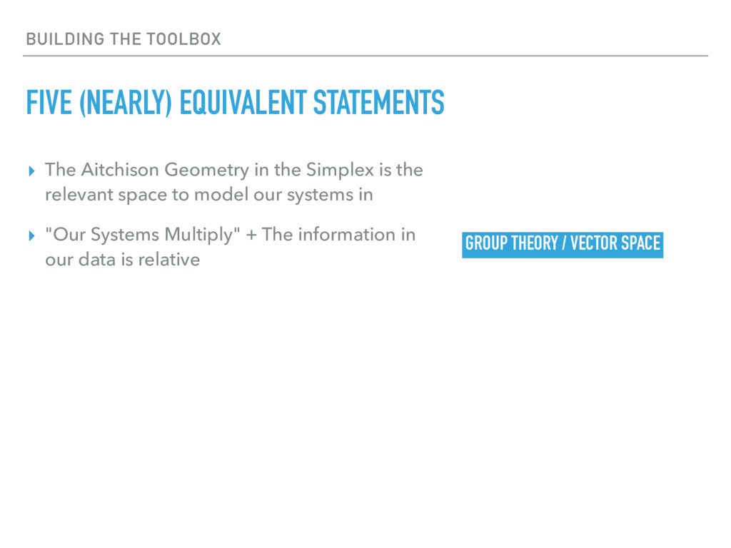
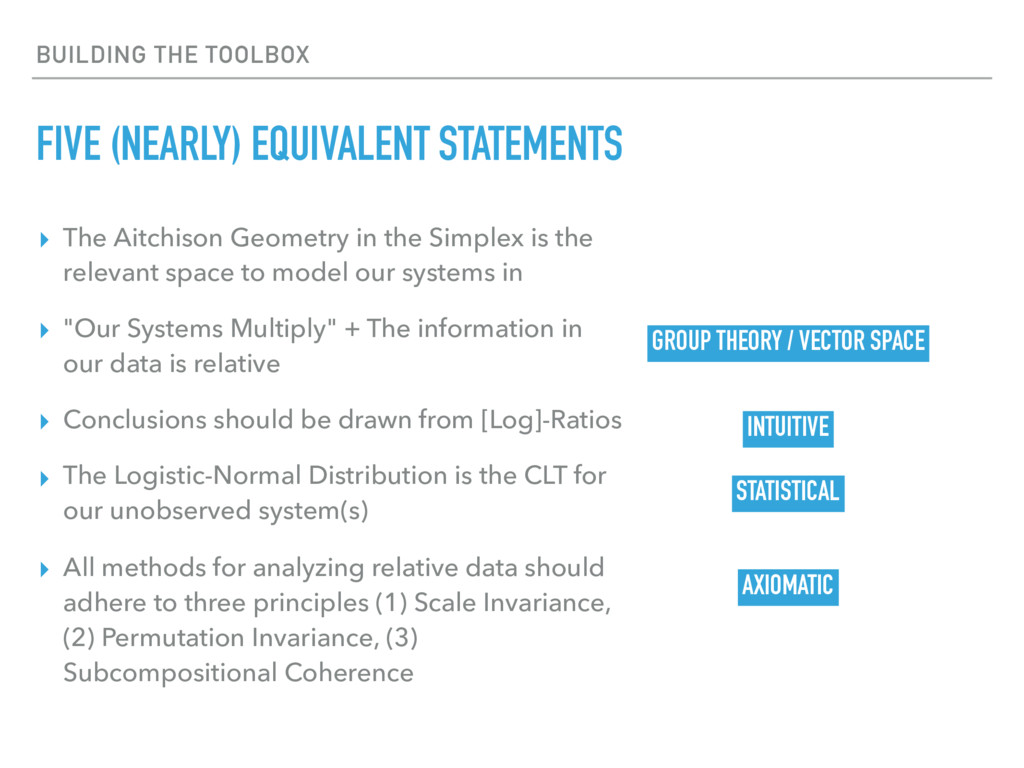
24. BUILDING THE TOOLBOX FIVE (NEARLY) EQUIVALENT STATEMENTS ▸ The Aitchison Geometry in the Simplex is the relevant space to model our systems in ▸ "Our Systems Multiply" + The information in our data is relative GROUP THEORY / VECTOR SPACE
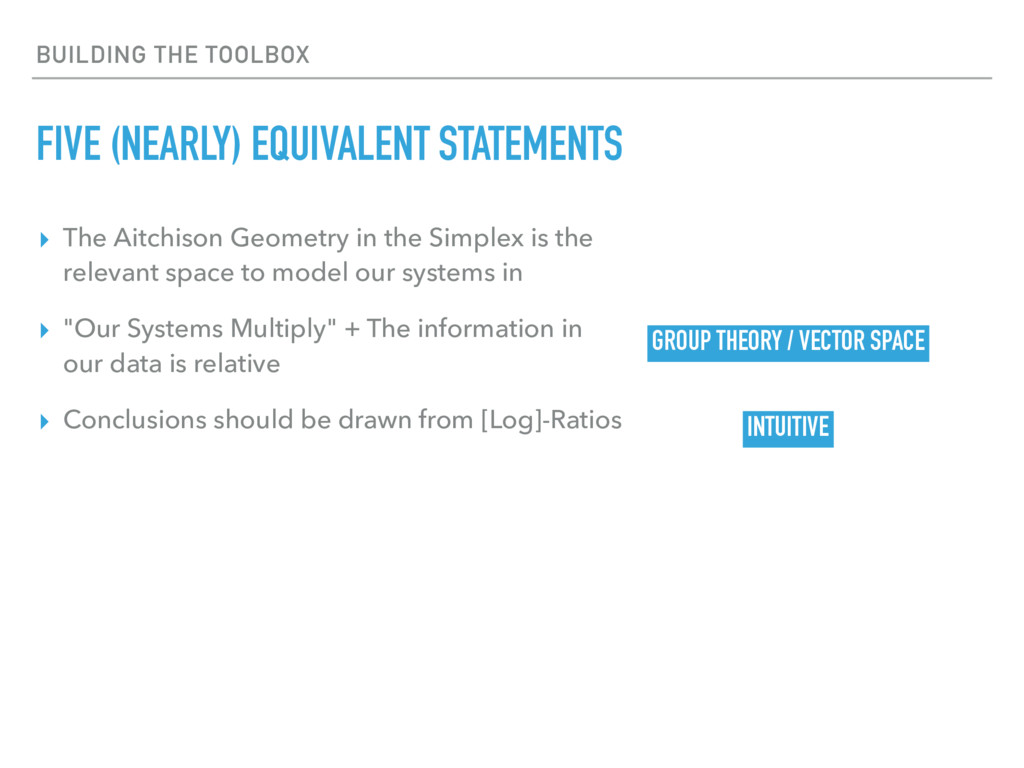
25. BUILDING THE TOOLBOX FIVE (NEARLY) EQUIVALENT STATEMENTS ▸ The Aitchison Geometry in the Simplex is the relevant space to model our systems in ▸ "Our Systems Multiply" + The information in our data is relative ▸ Conclusions should be drawn from [Log]-Ratios GROUP THEORY / VECTOR SPACE INTUITIVE
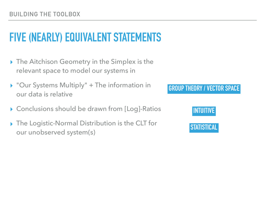
26. BUILDING THE TOOLBOX FIVE (NEARLY) EQUIVALENT STATEMENTS ▸ The Aitchison Geometry in the Simplex is the relevant space to model our systems in ▸ "Our Systems Multiply" + The information in our data is relative ▸ Conclusions should be drawn from [Log]-Ratios ▸ The Logistic-Normal Distribution is the CLT for our unobserved system(s) GROUP THEORY / VECTOR SPACE INTUITIVE STATISTICAL
27. BUILDING THE TOOLBOX FIVE (NEARLY) EQUIVALENT STATEMENTS ▸ The Aitchison Geometry in the Simplex is the relevant space to model our systems in ▸ "Our Systems Multiply" + The information in our data is relative ▸ Conclusions should be drawn from [Log]-Ratios ▸ The Logistic-Normal Distribution is the CLT for our unobserved system(s) ▸ All methods for analyzing relative data should adhere to three principles (1) Scale Invariance, (2) Permutation Invariance, (3) Subcompositional Coherence GROUP THEORY / VECTOR SPACE INTUITIVE STATISTICAL AXIOMATIC
28. MODELING GENERATIVE MODELING (LIKELIHOOD ONLY) Adapted from Hamady. et al., Nature Methods, 2008 Sample Collection 
 and Storage DNA Extraction
 PCR Amplification Sequencing
29. INTERPRETING THE MODEL MULTINOMIAL-LOGISTIC NORMAL (OR NORMAL ON THE SIMPLEX)
30. INTERPRETING THE MODEL
31. INTERPRETING THE MODEL PHYLOGENIC ISOMETRIC LOGRATIO (PHILR) TRANSFORM y2 * y1 * y2 * y1 * Lactobacillus Ruminococcus Bacteroides y1 * y2 * Lactobacillus Ruminococcus Bacteroides y1 * y2 * Community A Community B Bacteroides (%) Lactobacillus (%) Ruminococcus (%) Silverman, et al., eLife 2017 PHYLOGENETIC BALANCES ORTHONORMAL BASIS IN SIMPLEX DATA PROJECTED ONTO BASIS
32. INTERPRETING THE MODEL PHYLOGENIC ISOMETRIC LOGRATIO (PHILR) TRANSFORM y2 * y1 * y2 * y1 * Lactobacillus Ruminococcus Bacteroides y1 * y2 * Lactobacillus Ruminococcus Bacteroides y1 * y2 * Community A Community B Bacteroides (%) Lactobacillus (%) Ruminococcus (%) Silverman, et al., eLife 2017 PHYLOGENETIC BALANCES ORTHONORMAL BASIS IN SIMPLEX DATA PROJECTED ONTO BASIS
33. INTERPRETING THE MODEL WHY AN ORTHONORMAL BASIS? NON-ORTHONORMAL BASIS
34. INTERPRETING THE MODEL WHY AN ORTHONORMAL BASIS? NON-ORTHONORMAL BASIS
35. INTERPRETING THE MODEL WHY AN ORTHONORMAL BASIS? ORTHONORMAL BASIS
36. INTERPRETING THE MODEL WHY AN ORTHONORMAL BASIS? ORTHONORMAL BASIS
37. EXAMPLE APPLICATIONS
38. EXAMPLE APPLICATIONS: LONGITUDINAL ANALYSIS MODELING TIME-EVOLUTION WITH MALLARD θ0 θ1 θ2 ... θT True State with Biological Noise
39. EXAMPLE APPLICATIONS: LONGITUDINAL ANALYSIS MODELING TIME-EVOLUTION WITH MALLARD θ0 θ1 θ2 ... θT W1 W2 WT True State with Biological Noise
40. EXAMPLE APPLICATIONS: LONGITUDINAL ANALYSIS MODELING TIME-EVOLUTION WITH MALLARD θ0 θ1 θ2 ... θT η1 η2 ηT W1 W2 WT True State with Biological Noise Addition of Technical Noise
41. EXAMPLE APPLICATIONS: LONGITUDINAL ANALYSIS MODELING TIME-EVOLUTION WITH MALLARD θ0 θ1 θ2 ... θT η1 η2 ηT V1 V2 VT W1 W2 WT True State with Biological Noise Addition of Technical Noise
42. EXAMPLE APPLICATIONS: LONGITUDINAL ANALYSIS MODELING TIME-EVOLUTION WITH MALLARD θ0 θ1 Y1 θ2 Y2 ... θT YT η1 η2 ηT V1 V2 VT W1 W2 WT True State with Biological Noise Observed Counts Addition of Technical Noise
43. EXAMPLE APPLICATIONS: LONGITUDINAL ANALYSIS MODELING TIME-EVOLUTION WITH MALLARD θ0 θ1 Y1 θ2 Y2 ... θT YT η1 η2 ηT V1 V2 VT W1 W2 WT True State with Biological Noise Observed Counts Addition of Technical Noise ILR
44. EXAMPLE APPLICATIONS: LONGITUDINAL ANALYSIS MODELING TIME-EVOLUTION WITH MALLARD Y t ⇠ Multinomial(⇡t) ⇡t = ILR 1(⌘t ) ⌘t = F 0 t ✓t + ⌫t ⌫t ⇠ N ✓t = Gt✓t 1 + !t !t ⇠ N True State with Biological Noise Addition of Technical Noise Observed Counts θ0 θ1 Y1 θ2 Y2 ... θT YT η1 η2 ηT V1 V2 VT W1 W2 WT True State with Biological Noise Observed Counts Addition of Technical Noise ILR
45. EXAMPLE APPLICATIONS: LONGITUDINAL ANALYSIS A SIMPLE SIMULATION
46. EXAMPLE APPLICATIONS: LONGITUDINAL ANALYSIS A SIMPLE SIMULATION
47. EXAMPLE APPLICATIONS: LONGITUDINAL ANALYSIS RIKENELLACEAE RATIO CHANGES UPON STARVATION Balance Value
48. • • • • • • • • • • • • • • • • • • • • • • • • • • • • • • • • • • • • • • • • • • • • • • • • • • • • • • • • • • • • • • • • • • • • • • • • • • • • • • • • • • • • • • • • • • • • • • • • • • • • • • • • • • • • • • • • • • • • • • • • • • • • • • • • • • • • • • • • • • • • • • • • • • • • • • • • • • • • • • • • • • • • • • • • • • • • • • • • • • • • • • • • • • • • • • • • • • • • • • •• • • • • • • • • • • • • • • • • • • • • • • • • • • • • • • • • • • • • • • • • • • • • • • • • • • •• • • • • • • • • • • • • • • • • • • • • • • • • • • • • • • • • • • • • • • • • • • • • • • • • • • • • • • • • • • • • • • • Dosing Schedule Subject 16S8921 Subject 908 Subject Ai96 Subject J112526T Apr 17 Apr 24 0.0 0.1 0.2 0.3 0.00 0.25 0.50 0.75 1.00 0.00 0.25 0.50 0.75 1.00 0.00 0.25 0.50 0.75 0.00 0.25 0.50 0.75 EXAMPLE APPLICATIONS: COMPOSITIONAL CONTROL COMPOSITIONAL CONTROL OF ERYSIPELOTRICHACEAE 0.2 MG/25ML TID
 FORECAST • Stool from 4 human donors cultured ex vivo •2 week fixed and variable dosing trial •Hourly Sampling •Latent Matrix-Variate State Space Model with Non-Linear Transfer Function •Control based on minimizing expected loss over posterior forecasts
49. ACKNOWLEDGEMENTS ACKNOWLEDGEMENTS Duke University Lawrence David Sayan Mukherjee Rachael Bloom Heather Durand University de Girona Juan José Egozcue Vera Pawlowsky-Glahn MERCK Rachel Silverman Funding Duke Collaborative Quantitative Approaches to Problems in the Basic and Clinical Sciences 
 Duke MSTP NIH T32 xkcd.com StatsAtHome.com inschool4life Montana State 
 University Alex Washburne