Exploratory: An Introduction to Linear Regression

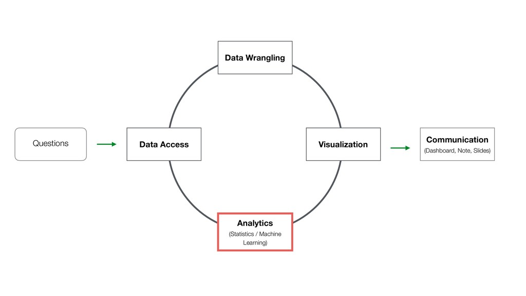
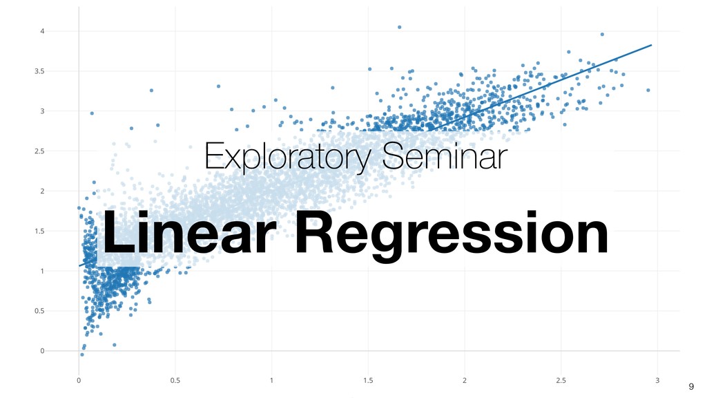
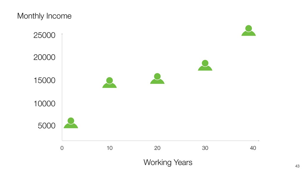
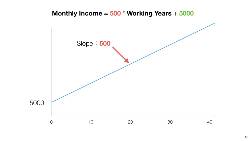
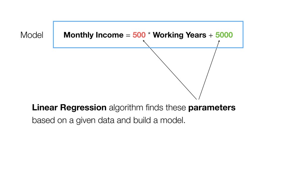
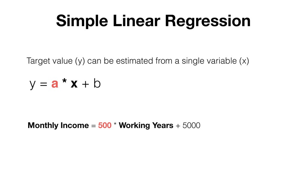
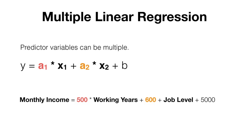
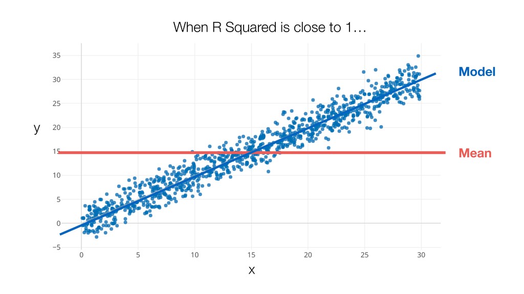
Linear Regression algorithm is considered as a basic algorithms, yet it is still one of the most popular algorithms in the world of data science because of its simplicity and applicability to many use cases.

Kan will be introducing the basic of Linear Regression algorithm and how to gain useful insights from the prediction model built by the algorithm in order.

Transcript

1. 1 Exploratory Seminar Linear Regression
2. EXPLORATORY
3. Kan Nishida co-founder/CEO Exploratory Summary Beginning of 2016, launched Exploratory, Inc. to democratize Data Science. Prior to Exploratory, Kan was a director of product development at Oracle leading teams for building various Data Science products in areas including Machine Learning, BI, Data Visualization, Mobile Analytics, Big Data, etc. While at Oracle, Kan also provided training and consulting services to help organizations transform with data. @KanAugust Speaker
4. Mission Make Data Science Available for Everyone
5. Data Science is not just for Engineers and Statisticians. Exploratory makes it possible for Everyone to do Data Science. The Third Wave
6. First Wave Second Wave Third Wave Proprietary Open Source UI & Programming Programming 2016 2000 1976 Monetization Commoditization Democratization Statisticians Data Scientists Democratization of Data Science Algorithms Experience Tools Open Source UI & Automation Business Users Theme Users
7. Questions Communication (Dashboard, Note, Slides) Data Access Data Wrangling Visualization Analytics (Statistics / Machine Learning) Exploratory Data Analysis
8. Questions Communication (Dashboard, Note, Slides) Data Access Data Wrangling Visualization Analytics (Statistics / Machine Learning)
9. 9 Exploratory Seminar Linear Regression
10. An Old and Basic regression algorithm, but due to its Simplicity it is still one of the most commonly used Statistical (or Machine) Learning algorithm. Linear Regression
11. Data 11
12. Employee Data
13. Monthly Income
14. Monthly Income
15. Questions 15
16. What is Monthly Income in this company? 16 Questions
17. Average of Monthly Income 17 $6,503
18. But… 18
19. Doesn’t Monthly Income varies? 19
20. $6,503 Average
21. $6,503 Variance Average $15,000 $1,000
22. What makes Monthly Income change and How? 22
23. Correlation 23
24. 24 Correlation A relationship where changes in one variable happen together with changes in another variable with a certain rule.
25. Strong Negative Correlation No Correlation Strong Positive Correlation 0 1 -1 -0.5 0.5 Correlation
26. 26 Age Monthly Income The bigger the Age is, the bigger the Monthly Income is. Correlation
27. 27 Why Correlation is Important?
28. 28 Variance Average (Mean) $20,000 $1,000
29. 29 Variance $20,000 $1,000 Monthly Income
30. 30 How much the income would be in this company? $20,000 $1,000 Monthly Income Variance
31. 31 Uncertainty $20,000 $1,000 Monthly Income How much the income would be in this company? Variance
32. 32 0 30 20 If we can find a correlation between Monthly Income and Working Years… 10 $20,000 $1,000 Working Years Monthly Income
33. 33 0 30 20 10 $20,000 $1,000 Working Years If Working Years is 20 years, Monthly Income would be around $15,000. $15,000 Monthly Income
34. 34 5000 0 30 20 Working Years Correlation Variance 100 $20,000 $1,000 $15,000 Correlation reduces Uncertainty caused by Variance. Monthly Income
35. If we can find strong correlations, it makes it easier to explain how Monthly Income changes and to predict what Monthly Income will be.
36. Correlation is not equal to Causation. Causation is a special type of Correlation. If we can confirm a given Correlation is Causation, then we can control the outcome.
39. Is finding Correlation enough? 39
40. • How much of the change in Monthly Income we can expect by a change in Working Years? • If there is, how big is it? Is it Strong enough that we should pay attention to it? • How much of the variance can it explain? Given that we find a correlation between two variables…
41. We can build Linear Regression models to answer these questions.
42. Linear Regression Basics 42
43. 43 Monthly Income 5000 10000 15000 25000 20000 Working Years 40 20 10 0 30
44. Want to find a simple pattern that can explain both the given data and the data we don’t have at hands. 44
45. 45 500ສ ۈଓ೥਺ 40೥ 20೥ 10೥ ೖࣾ 30೥ څྉ 1000ສ 1500ສ 2000ສ
46. 46 Draw a line to make the distance between the actual values and the line to be minimal. 40 20 10 0 30 5000 10000 15000 25000 20000
47. 47 40 20 10 0 30 5000 10000 15000 25000 20000 Monthly Income = 500 * Working Years + 5000
48. 48 5000 Slopeɿ500 40 20 10 0 30 Monthly Income = 500 * Working Years + 5000
49. 49 5000 40 20 10 0 30 Y Intercept Monthly Income = 500 * Working Years + 5000
50. Linear Regression algorithm finds these parameters based on a given data and build a model. Model Monthly Income = 500 * Working Years + 5000
51. Target value (y) can be estimated from a single variable (x) y = a * x + b Simple Linear Regression Monthly Income = 500 * Working Years + 5000
52. Predictor variables can be multiple. y = a1 * x1 + a2 * x2 + b Multiple Linear Regression Monthly Income = 500 * Working Years + 600 + Job Level + 5000
53. 53 40 20 10 0 30 5000 10000 15000 25000 20000 With real world data, it never predicts perfectly. Residuals
54. 54 Let’s try
56. 56 Select TotalWorkingYears
58. 58 MonthlyIncome = 468 * TotalWorkingYears + 1228
59. • Coefficient (Slope) • P Value • R-Squared 59 Basics of Linear Regression
60. • Coefficient (Slope) • P Value • R-Squared 60 Basics of Linear Regression
61. Monthly Income = 500 * Working Years + 5000 Slope Intercept
62. 62 Working Years 4 2 1 0 3 Monthly Income = 500 * Working Years + 5000 5000 5500 6000 6500 Slopeɿ500 One year increase in Working Years will increase Monthly Income for $500.
63. 63 5000 Slopeɿ1000 5500 6000 6500 7000 Working Years 4 2 1 0 3 Monthly Income = 1000 * Working Years + 5000 One year increase in Working Years will increase Monthly Income for $1000.
64. 64 Working Years 4 2 1 0 3 Monthly Income = -500 * Working Years + 6500 5000 5500 6000 6500 Slopeɿ-500 One year increase in Working Years will decrease Monthly Income for $500.
65. 65 Working Years 4 2 1 0 3 Monthly Income = 0 * Working Years + 5500 5000 5500 6000 6500 Slopeɿ0 Regardless of the values in Working Years, Monthly Income is always $5,500.
66. 66 Working Years 4 2 1 0 3 Monthly Income = 0 * Working Years + 5500 5000 5500 6000 6500 Slopeɿ0 Working Years and Monthly Income are independent.
67. 67 Working Years Monthly Income Independent No effect on the other side.
68. 68 MonthlyIncome = 468 * TotalWorkingYears + 1228
69. 69 1228 1500 2000 2500 Slopeɿ468 MonthlyIncome = 468 * TotalWorkingYears + 1228 1000 Working Years 4 2 1 0 3
70. 70 MonthlyIncome = 468 * TotalWorkingYears + 1228 1696 1500 2000 2500 1000 Working Years 4 2 1 0 3
71. 71 Monthly Income Working Years vs. Numeric Numeric
72. 72 Numeric Numeric
73. 73 Department vs. Category Numeric Monthly Income
74. 74 Category Numeric
76. 76 Compare to Base Level
77. 77 Summary Tab Coefficient Tab
78. 78 Name Sales HR Peter 1 0 Maria 0 1 Jane 1 0 Kan 0 0 Name Department Peter Sales Maria HR Jane Sales Kan R&D As part of the model building, categorical variables are expanded to multiple columns so that each category has its own column with values being either 0 or 1.
79. 79 If Department is SalesɺSales is 1ɺHR is 0. Name Sales HR Peter 1 0 Maria 0 1 Jane 1 0 Kan 0 0
80. 80 If Department is R&D (Base Level), both Sales & HR are 0. Name Sales HR Peter 1 0 Maria 0 1 Jane 1 0 Kan 0 0
82. 82 Sales department is $678 higher compared to R&D department.
83. • Coefficient (Slope) • P Value • R-Squared 83 Basics of Linear Regression
84. • Null Hypothesis : A given variable has nothing to do with the changes in the target variable. • We can use P Value as a guide to decide if we can reject Null Hypothesis. Statistical Test on Coefficient
85. Assuming Null Hypothesis, a Probability of getting the observed effect. 85 P Value
86. 86 Monthly Income Working Years vs.
89. 89 Working Years Monthly Income Null Hypothesis Independent
90. 90 Monthly Income = 467 * Working Years + 1227
91. 91 Coefficient for Working Years is 0 Null Hypothesis Monthly Income = 0 * Working Years + 1227
93. 93 P Value is 1ˋ (0.01). Very rare to observe this effect by random chance, we can accept that Monthly Income and Working Years are correlated.
94. 94 Correlated Working Years Monthly Income
95. 95 Monthly Income Distance from Work vs.
98. 98 Distance Monthly Income Null Hypothesis Independent
99. 99 Monthly Income = -9 * Distance + 6593
100. 100 Coefficient for Distance is 0 Null Hypothesis Monthly Income = 0 * Distance + 6593
102. 102 P Value is 51ˋ (0.51). It’s often to observe this effect by random chance, we can’t conclude that Monthly Income and Working Years are correlated.
103. 103 Can’t conclude they are correlated. Distance Monthly Income
104. Why not Significant? • The difference is small. • The data is small. 104
105. P Value Confidence Interval or
106. 106 Working Years Monthly Income ?
107. Coefficient is 467, but Confidence Interval is between 448 and 487. The true Coefficient should be included in this range at 95% probability. The coefficient is most likely not 0.
108. 108 Working Years 4 2 1 0 3 Monthly Income = 0 * Working Years + 5500 5000 5500 6000 6500 Slopeɿ0 Regardless of the values in Working Years, Monthly Income is always $5,500. If the coefficient was 0 …
109. 1227 The data is far from the flat!
110. 110 They are correlated. Working Years Monthly Income
111. 111 How about Distance? Distance Monthly Income ?
112. 0 Coefficient is -9, but Confidence Interval is between -39 and 19. The true Coefficient should be included in this range at 95% probability. The coefficient could be 0.
113. 113 Distance 4 2 1 0 3 Monthly Income = 0 * Distance + 6593 5000 5500 6000 6500 Slopeɿ0 Regardless of the values in Distance, Monthly Income is always $6,593.
114. Coefficient 0 means… 6593
115. 115 Can’t conclude they are correlated. Distance Monthly Income
116. • Coefficient (Slope) • P Value • R-Squared 116 Basics of Linear Regression
117. R Squared • How good does the model perform compared to a null model? • It can be between 0 and 1, 1 being the highest.
118. When R Squared is high… When R Squared is low… Let's take a look at High and Low scenarios.
119. When R Squared is close to 1… Mean Model x y
120. Mean Let’s look into this point. x y Model
121. Mean Most of the variability of the data is explained by the model. x y Model
122. Mean The part between the prediction and the dot is not explained by the model. The part between the prediction and the mean is explained by the model. x y Model
123. When R Squared is close to 0… Mean Let’s look into this dot. x y Model
124. Mean Only small part of the variability of the data is explained by the model. x y Model
125. The part between the prediction and the dot is not explained by the model. The part between the prediction and the mean is explained by the model. Mean x y Model
126. R Squared is the ratio of variability of the target variable values that is explained by the model. When R Squared is high… When R Squared is low…
127. 127 40 20 10 0 30 5000 10000 15000 25000 20000 Working Years Monthly Income
128. 128 Average 100% 60% 40 20 10 0 30 Working Years 5000 10000 15000 25000 20000 Monthly Income
129. 60% of the Monthly Income’s variance from the mean can be explained by Working Years. In order to explain the remaining 40% we need to go find other variables.
130. More Questions…
131. • Other variables are correlated, too. One variable changes while another variable changes at the same timing (Age vs. Working Years) • Want to know the independent effect of one variable alone. • How the variable effect on another variable might be different in different group of data. Want to compare the effects among the groups.
132. 132 Age Monthly Income Working Years
133. Q & A