Introduction to Time Series Forecasting with Prophet

- Introduction to Prophet
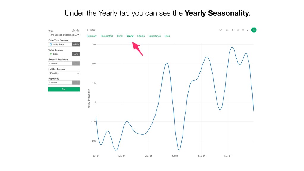
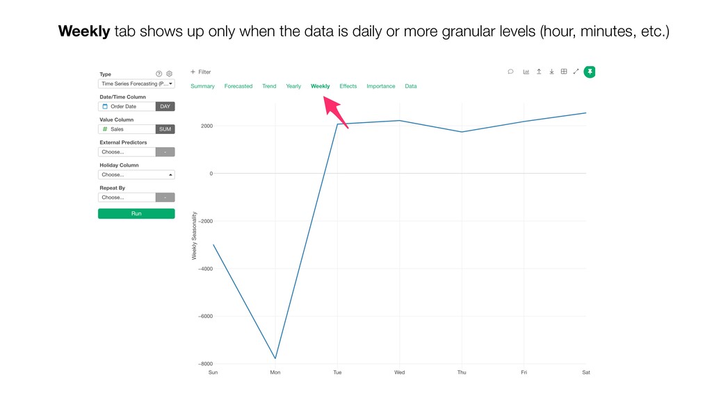
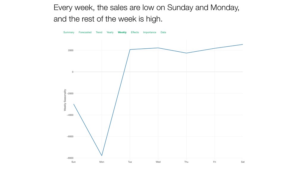
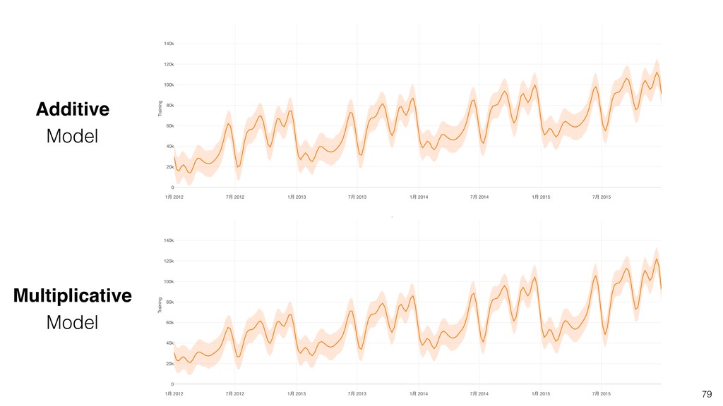
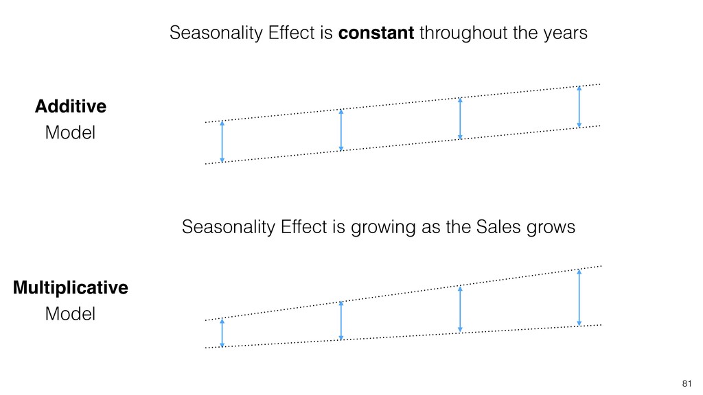
- Seasonality and Additive/Multiplicative Modes
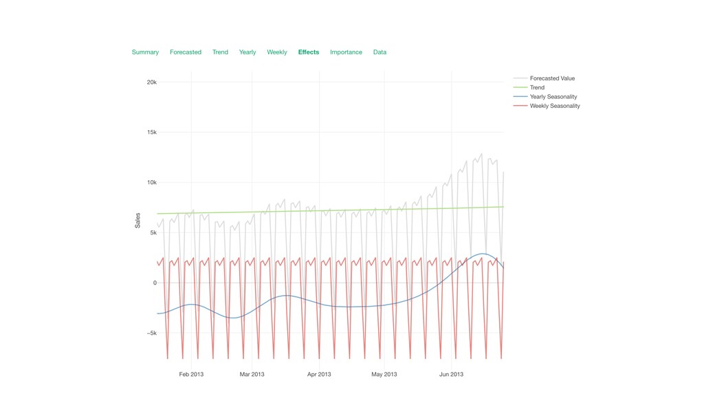
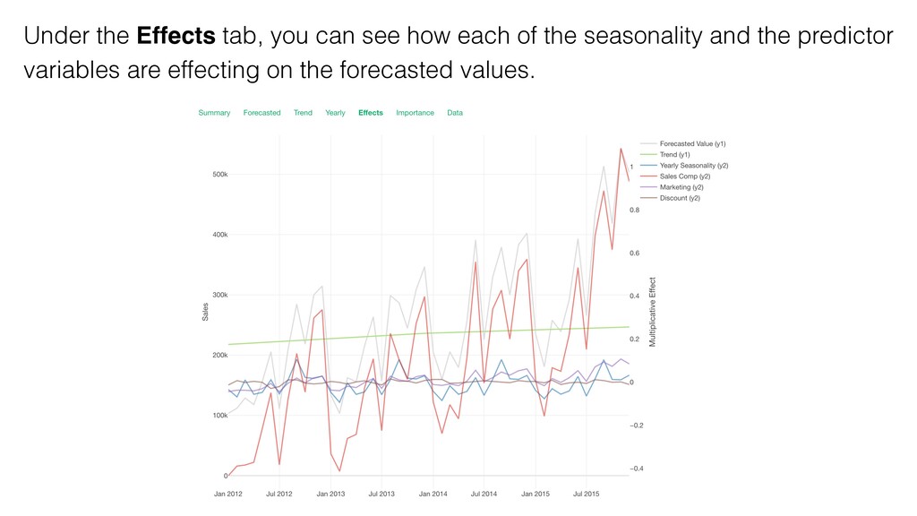
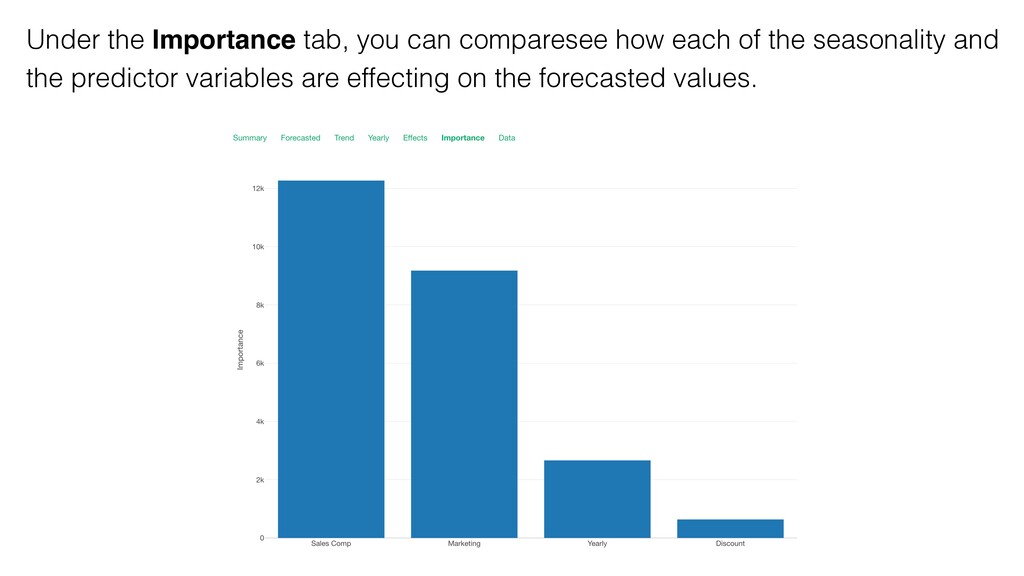
- Variable Importance / Effects
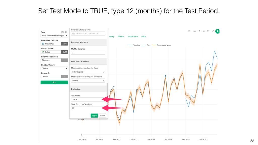
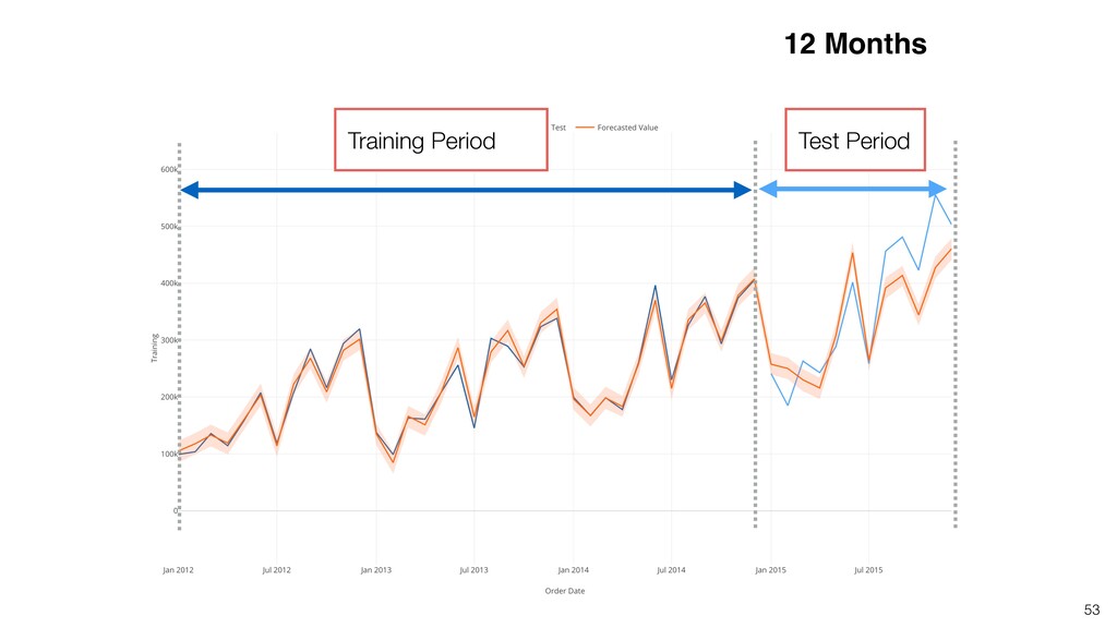
- Test Mode and Evaluation of the Model
- External Variables (Extra Regressor)

Transcript

1. Exploratory Seminar #25 Time Series Forecasting with Prophet
2. EXPLORATORY
3. Kan Nishida CEO/co-founder Exploratory Summary Beginning of 2016, launched Exploratory, Inc. to democratize Data Science. Prior to Exploratory, Kan was a director of product development at Oracle leading teams for building various Data Science products in areas including Machine Learning, BI, Data Visualization, Mobile Analytics, Big Data, etc. While at Oracle, Kan also provided training and consulting services to help organizations transform with data. @KanAugust Speaker
4. Mission Democratize Data Science
5. Data Science is not just for Engineers and Statisticians. Exploratory makes it possible for Everyone to do Data Science. The Third Wave
6. First Wave Second Wave Third Wave Proprietary Open Source UI & Programming Programming 2016 2000 1976 Monetization Commoditization Democratization Statisticians Data Scientists Democratization of Data Science Algorithms Experience Tools Open Source UI & Automation Business Users Theme Users
7. Questions Communication Data Access Data Wrangling Visualization Analytics (Statistics / Machine Learning) Data Analysis Data Science Workflow
8. Questions Communication (Dashboard, Note, Slides) Data Access Data Wrangling Visualization Analytics (Statistics / Machine Learning) Data Analysis ExploratoryɹModern & Simple UI
9. Exploratory Seminar #25 Time Series Forecasting with Prophet
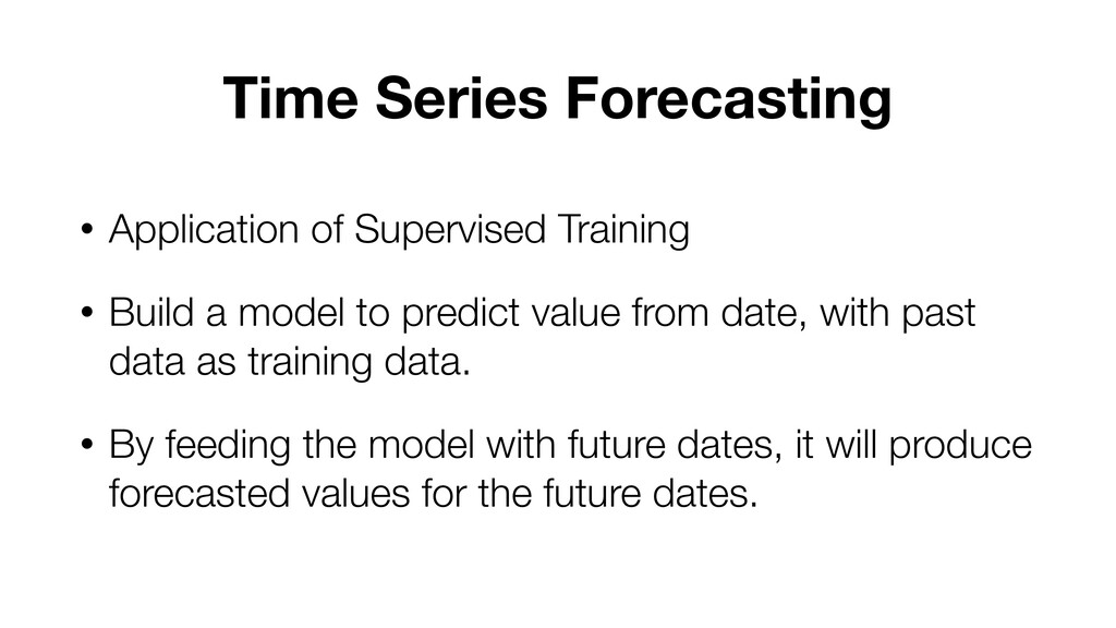
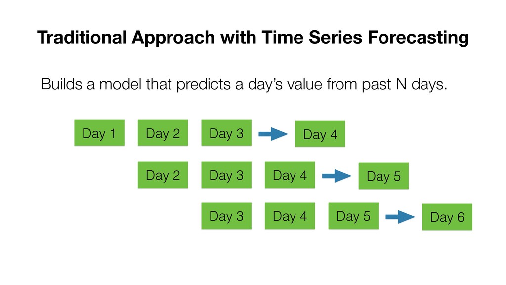
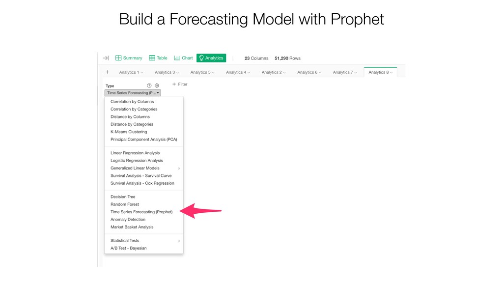
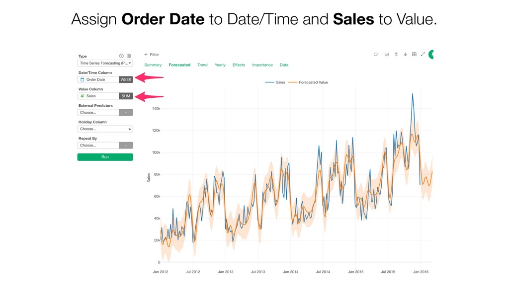
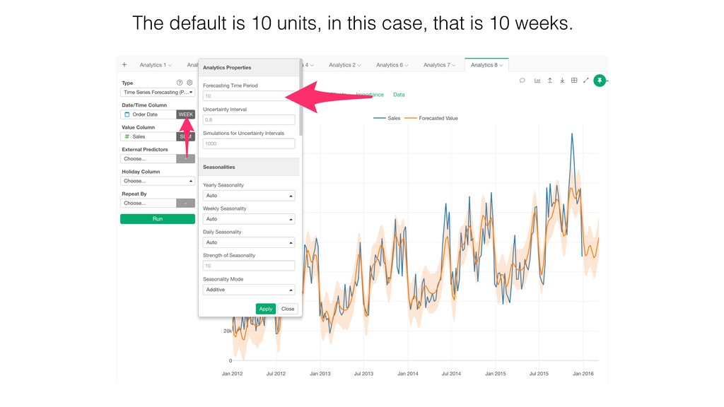
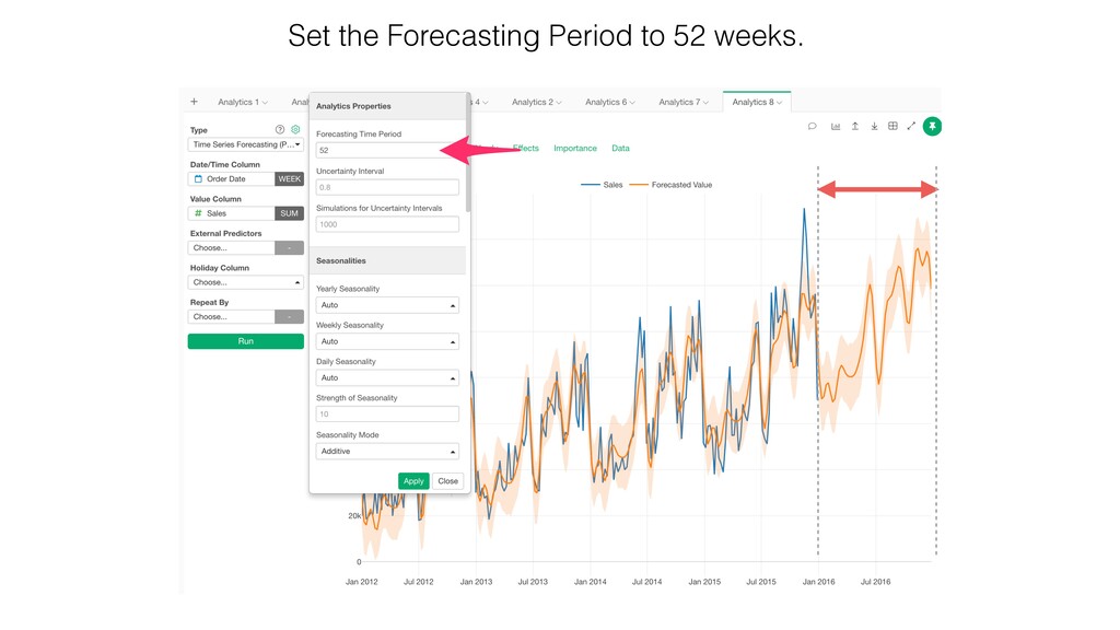
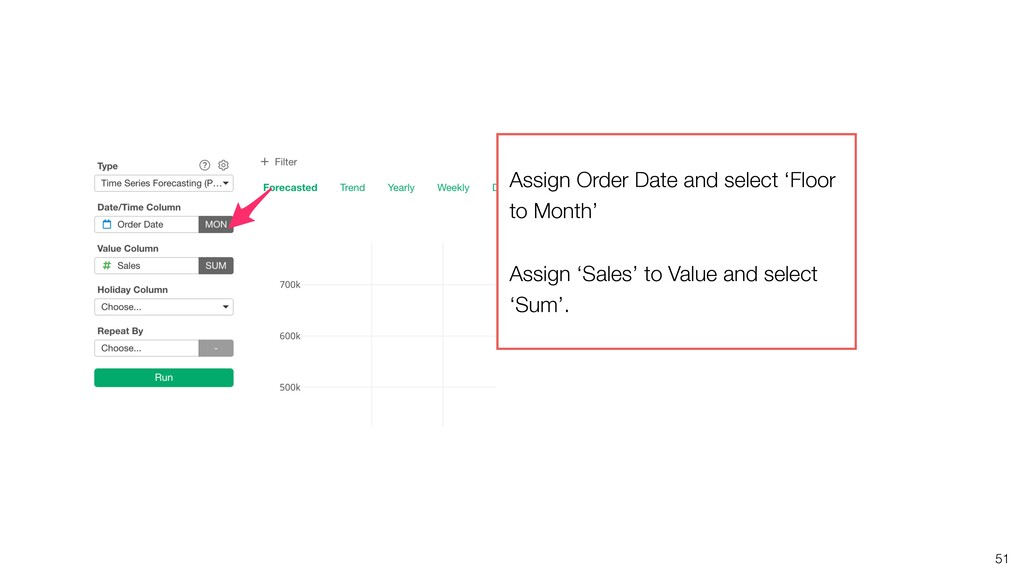
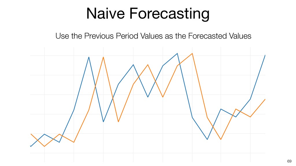
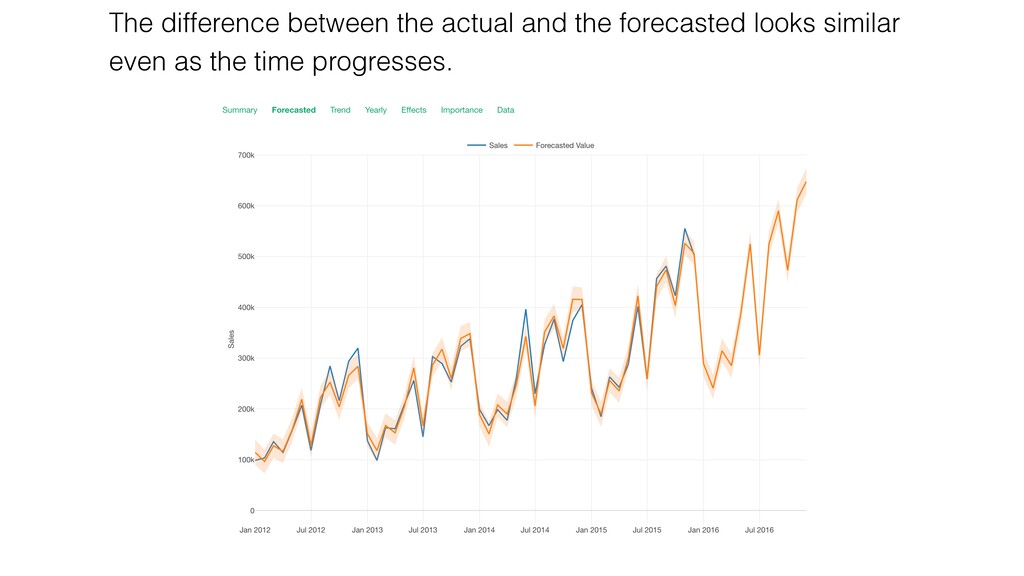
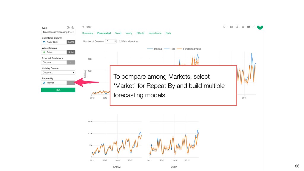
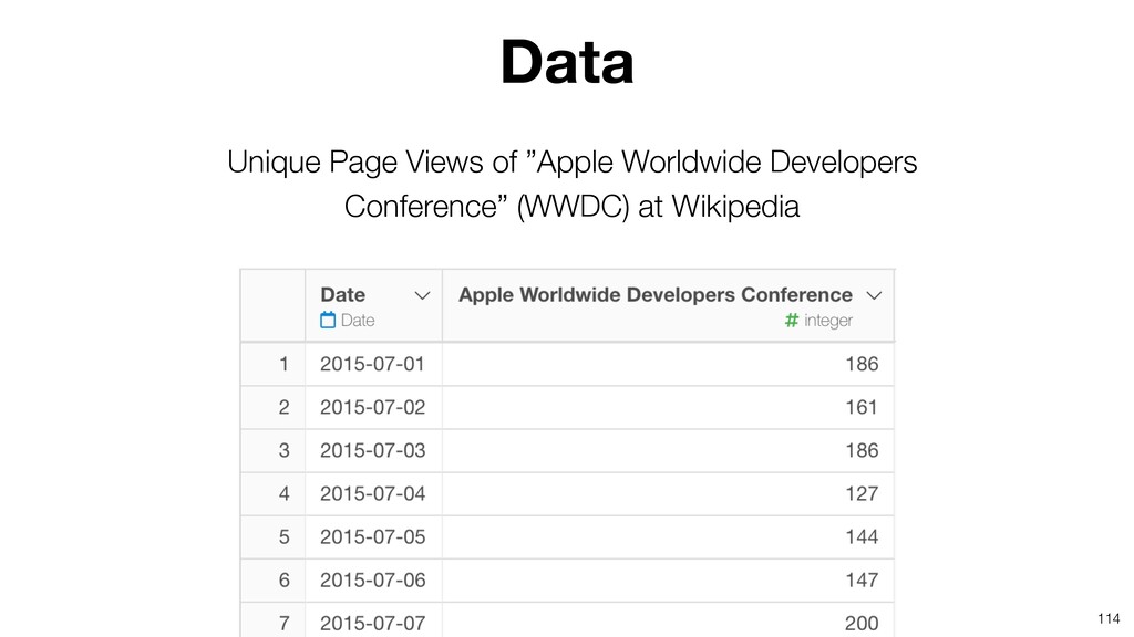
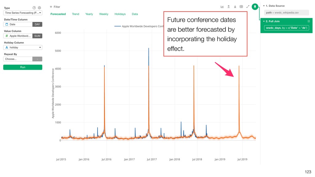
10. • Application of Supervised Training • Build a model to predict value from date, with past data as training data. • By feeding the model with future dates, it will produce forecasted values for the future dates. Time Series Forecasting
11. Builds a model that predicts a day’s value from past N days. Traditional Approach with Time Series Forecasting Day 1 Day 2 Day 3 Day 4 Day 2 Day 3 Day 4 Day 5 Day 3 Day 4 Day 5 Day 6
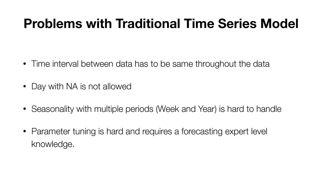
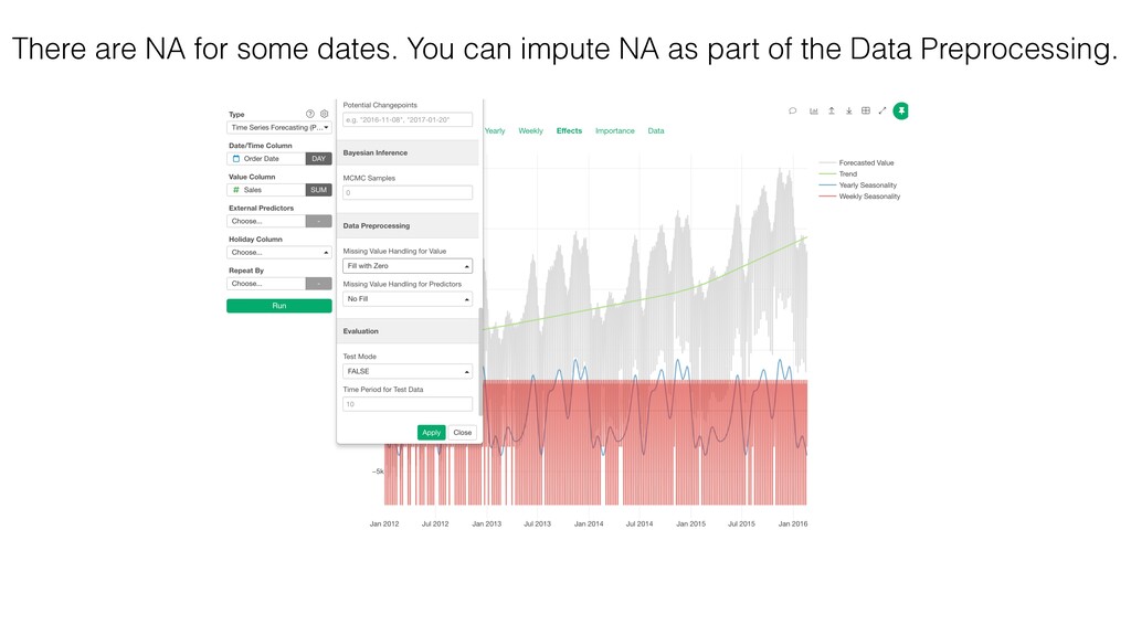
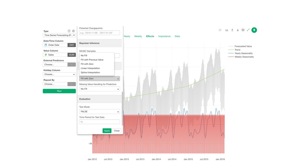
12. • Time interval between data has to be same throughout the data • Day with NA is not allowed • Seasonality with multiple periods (Week and Year) is hard to handle • Parameter tuning is hard and requires a forecasting expert level knowledge. Problems with Traditional Time Series Model
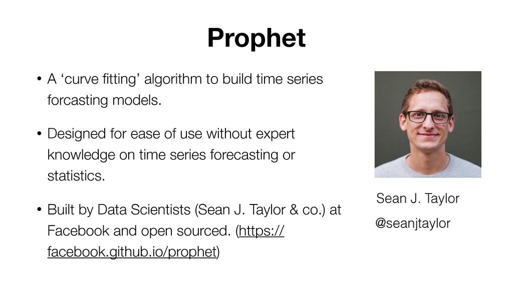
13. • A ‘curve fitting’ algorithm to build time series forcasting models. • Designed for ease of use without expert knowledge on time series forecasting or statistics. • Built by Data Scientists (Sean J. Taylor & co.) at Facebook and open sourced. (https:// facebook.github.io/prophet) Prophet Sean J. Taylor @seanjtaylor
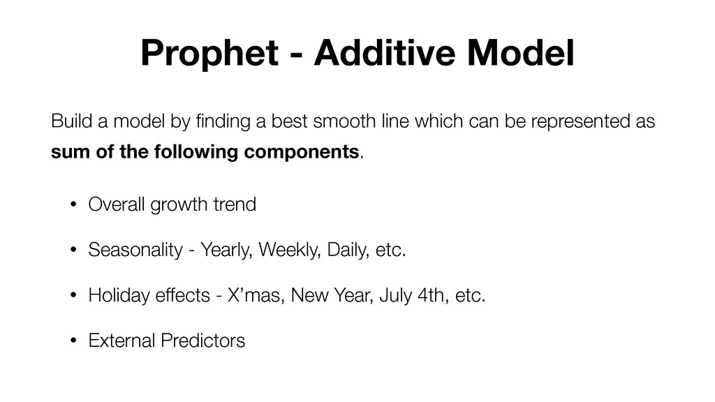
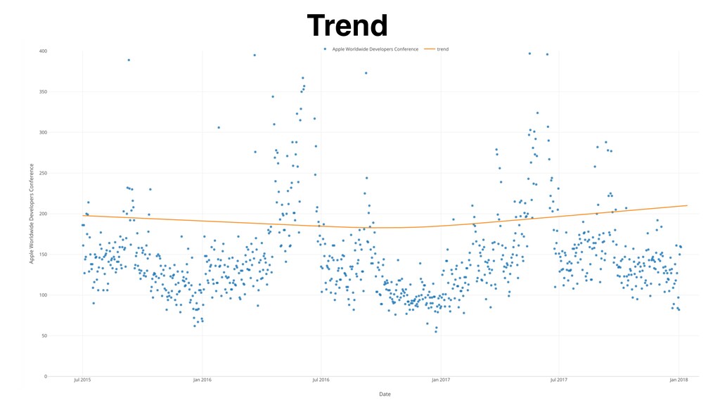
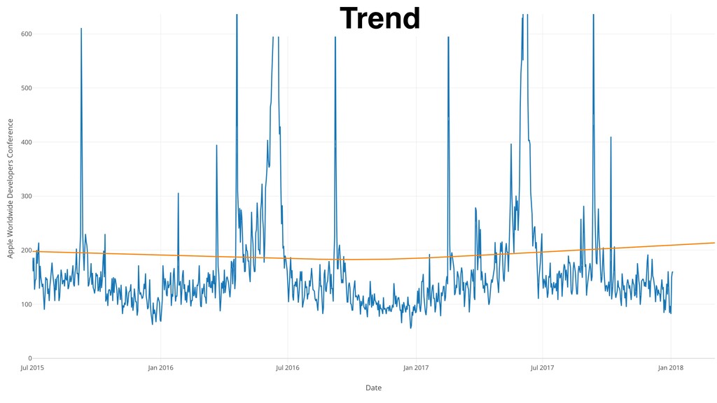
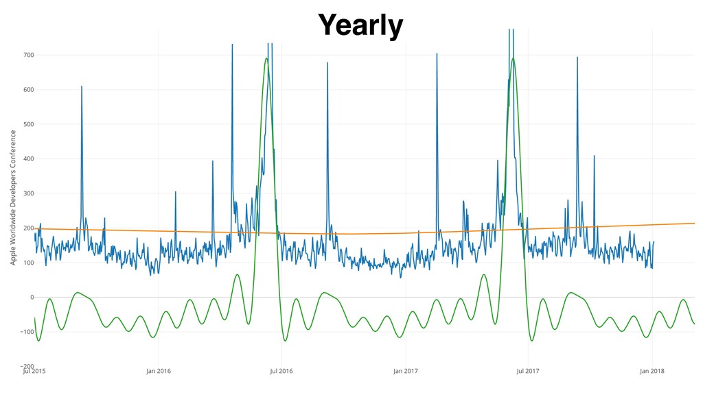
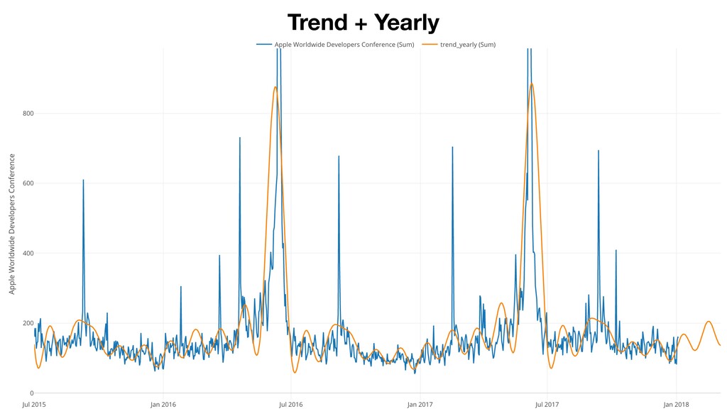
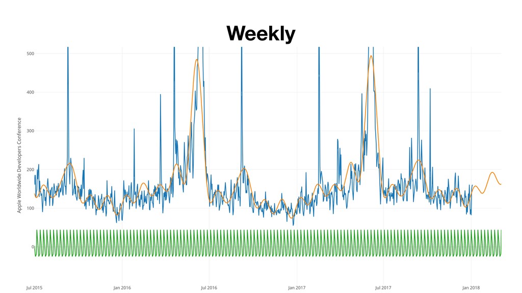
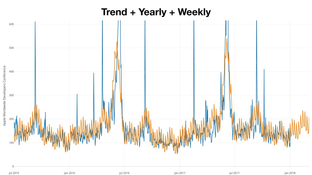
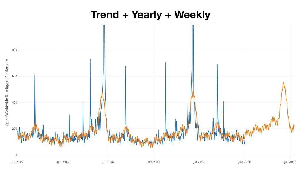
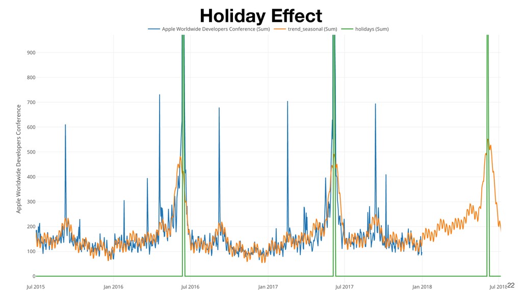
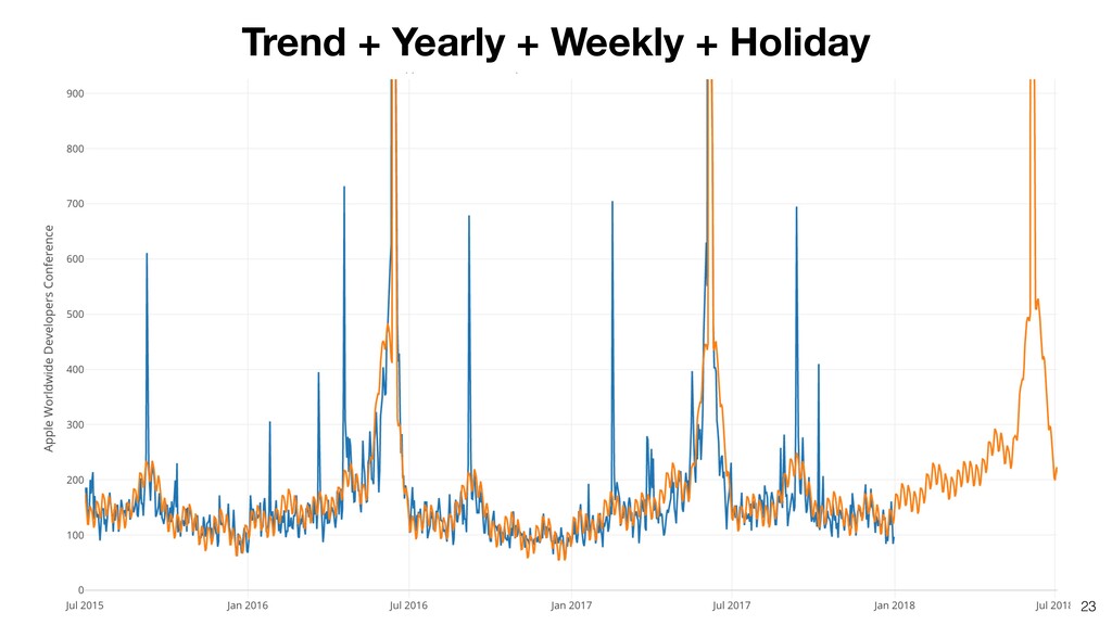
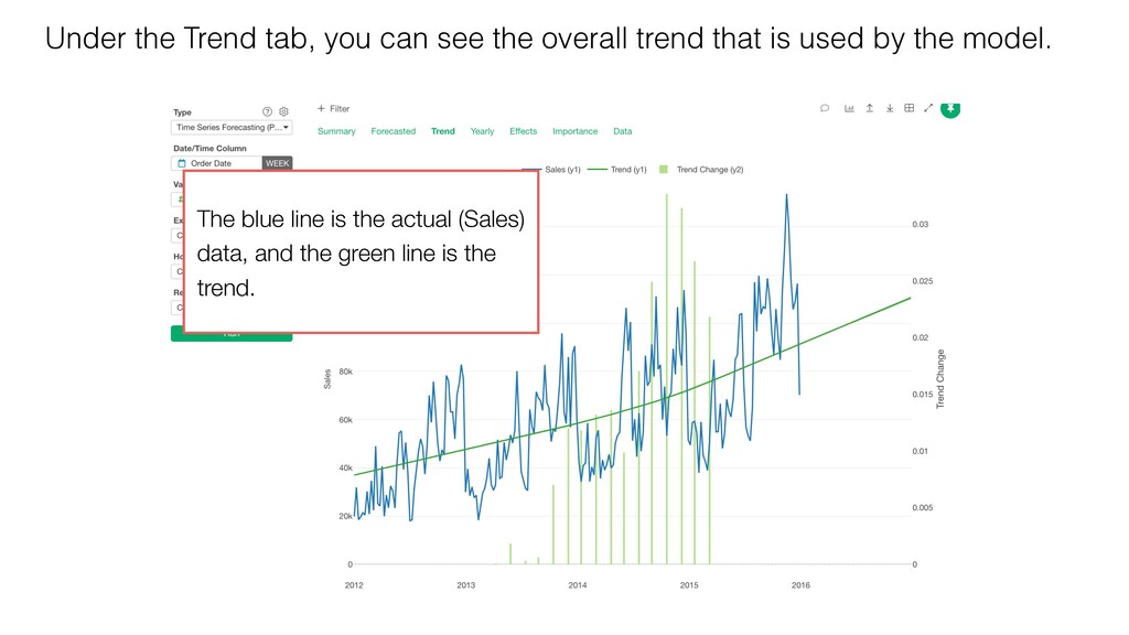
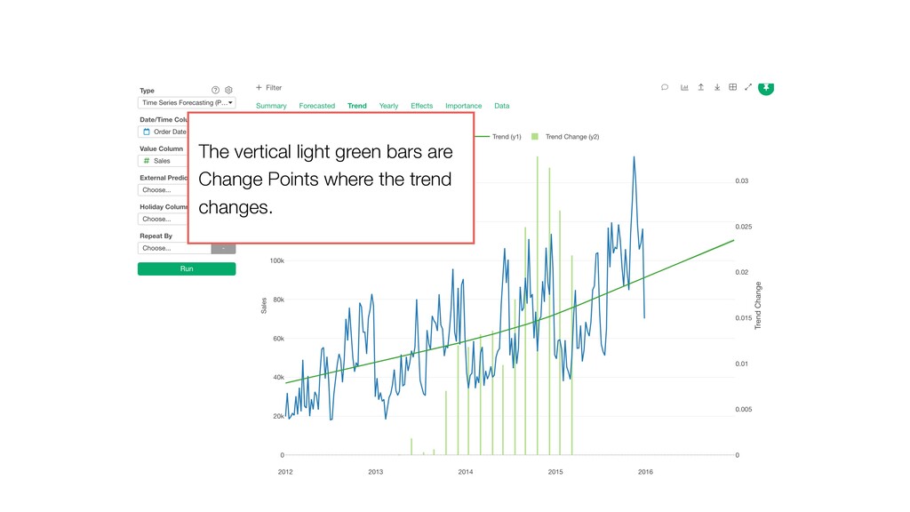
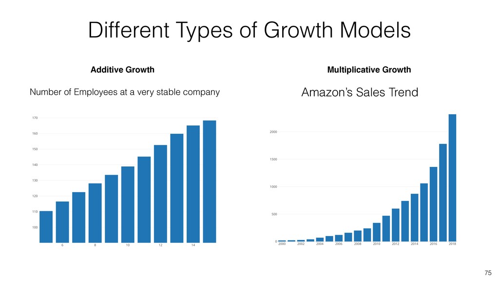
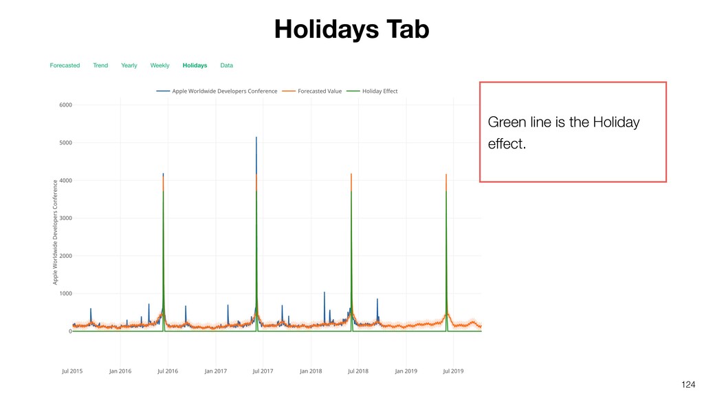
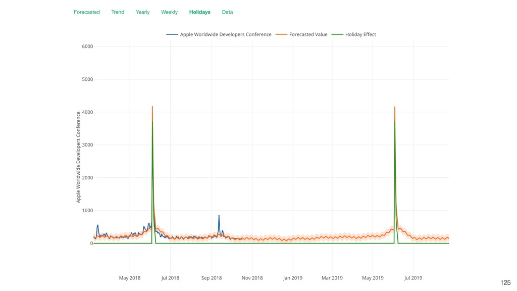
14. Build a model by finding a best smooth line which can be represented as sum of the following components. • Overall growth trend • Seasonality - Yearly, Weekly, Daily, etc. • Holiday effects - X’mas, New Year, July 4th, etc. • External Predictors Prophet - Additive Model
15. Trend
16. Trend
17. Yearly
18. Trend + Yearly
19. Weekly
20. Trend + Yearly + Weekly
21. 21 Trend + Yearly + Weekly
22. 22 Holiday Effect
23. 23 Trend + Yearly + Weekly + Holiday
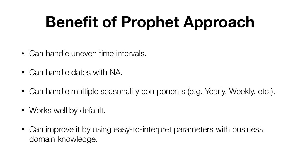
24. • Can handle uneven time intervals. • Can handle dates with NA. • Can handle multiple seasonality components (e.g. Yearly, Weekly, etc.). • Works well by default. • Can improve it by using easy-to-interpret parameters with business domain knowledge. Benefit of Prophet Approach
25. Let’s do it!
26. Sales Data
27. Weekly Sales Trend
28. Build a Forecasting Model with Prophet
29. Assign Order Date to Date/Time and Sales to Value.
30. The blue line is the actual data (Sales), and the orange line is the forecasted data.
31. The last area is the forecasted period where there is no actual data.
32. The default is 10 units, in this case, that is 10 weeks.
33. Set the Forecasting Period to 52 weeks.
34. Under the Trend tab, you can see the overall trend that is used by the model. The blue line is the actual (Sales) data, and the green line is the trend.
35. The vertical light green bars are Change Points where the trend changes.
36. Under the Yearly tab you can see the Yearly Seasonality.
37. Every year, the sales doesn’t pick up until June, then it goes down in July.
38. Weekly tab shows up only when the data is daily or more granular levels (hour, minutes, etc.)
39. Every week, the sales are low on Sunday and Monday, and the rest of the week is high.
40. Data Pre-Processing NA Data Handling
41. Somehow, the weekly seasonality doesn’t repeat exactly the same…
42. Somehow, the weekly seasonality doesn’t repeat exactly the same…
43. There are NA for some dates. You can impute NA as part of the Data Preprocessing.
46. Under the Importance tab, you can see which seasonality has more effect on the forecasting outcome.
47. 47 Evaluating Forecasting Model
48. • Keep the latest part of past data as test data • Forecast the test data period with the data before the test data period • Estimate the forecast Backtesting
49. Split the data into two sections. 49 Training Period Test Period
50. 50 Training Period Test Period Build a model with the training data and forecast for the test period. Compare the forecasted values against the actual values in the test period.
51. 51 Assign Order Date and select ‘Floor to Month’ Assign ‘Sales’ to Value and select ‘Sum’.
52. 52 Set Test Mode to TRUE, type 12 (months) for the Test Period.
53. 53 Training Period Test Period 12 Months
54. Since the forecasting model is built based on the training data, the forecasted values (Orange) and the actual values (Blue) are usually very close. 54
55. 55 Evaluate the model based on how much difference there is between the forecasted values and the actual values in the Test period.
56. Evaluation Metrics under Summary tab 56
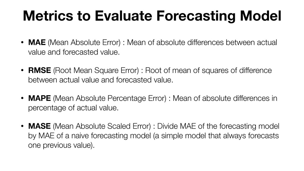
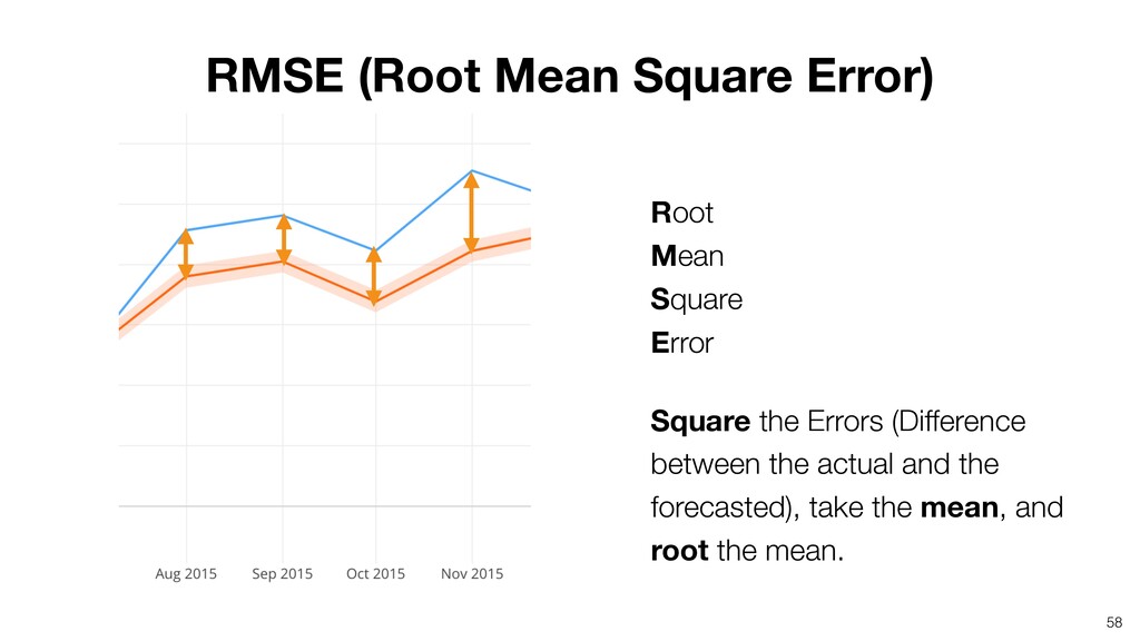
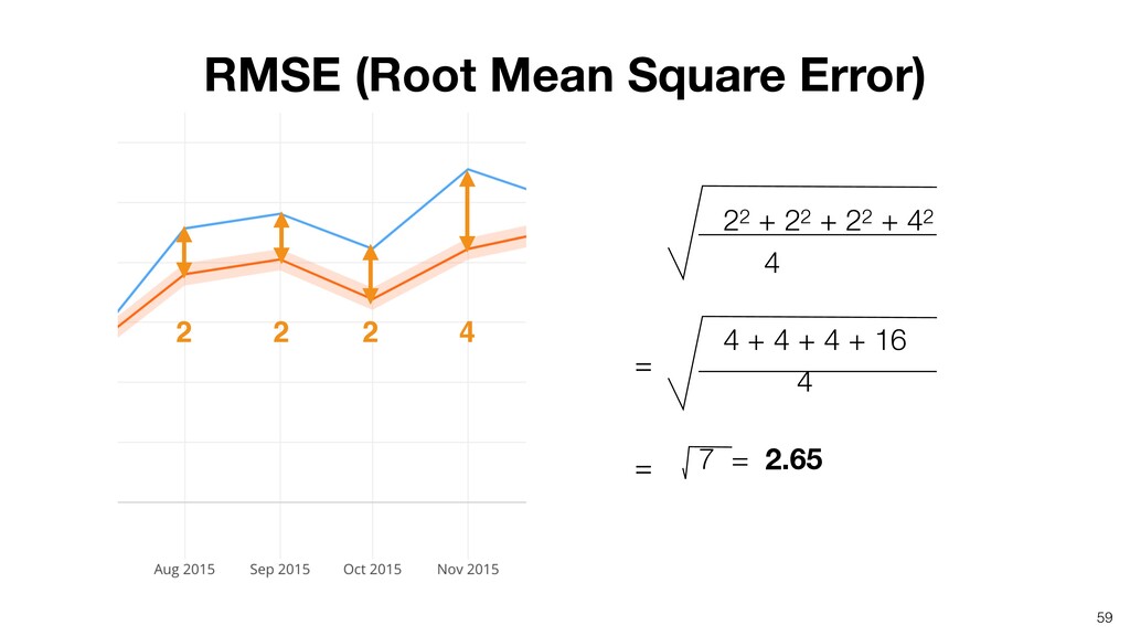
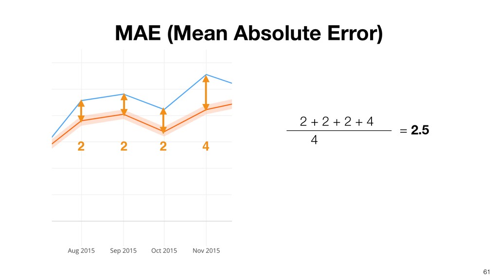
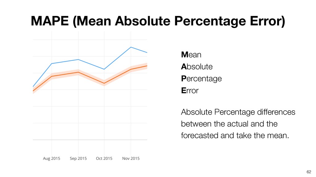
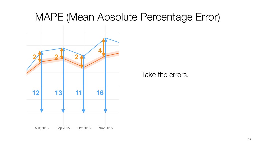
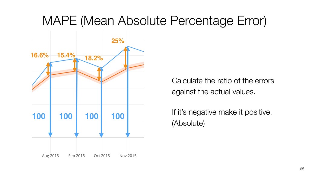
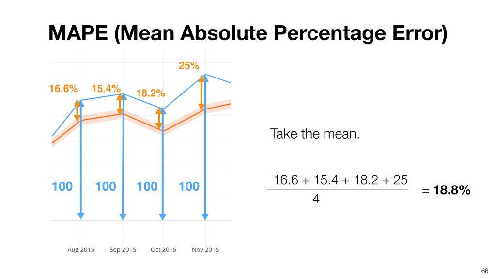
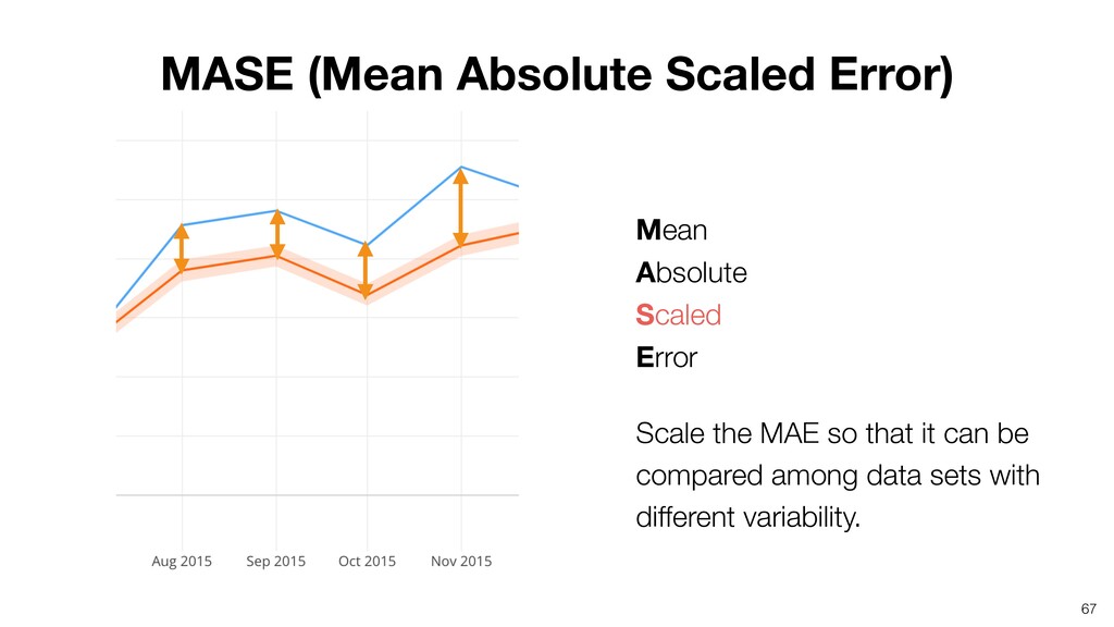
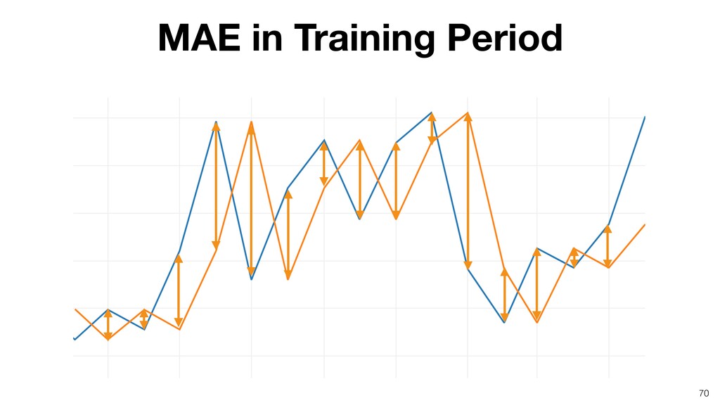
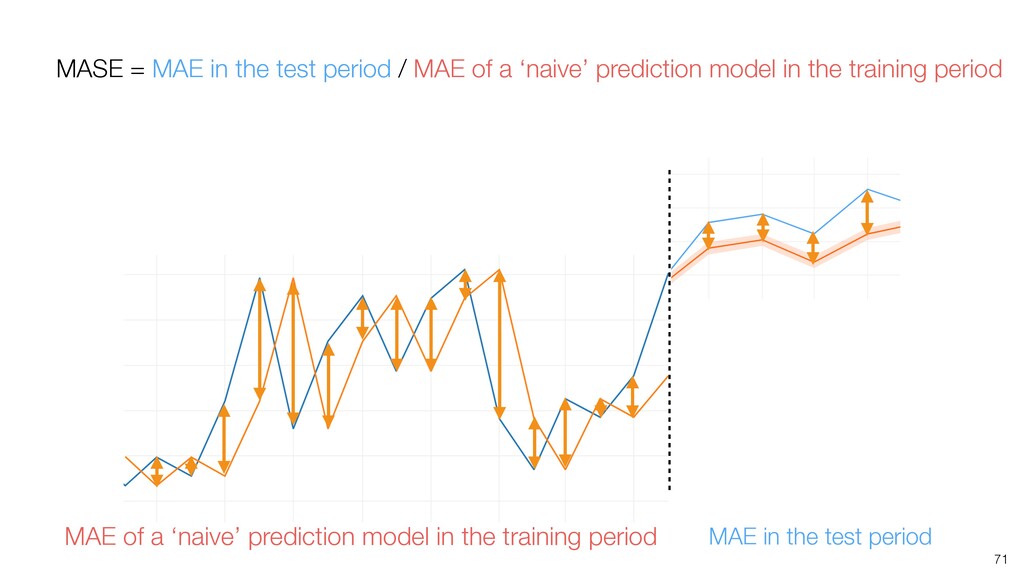
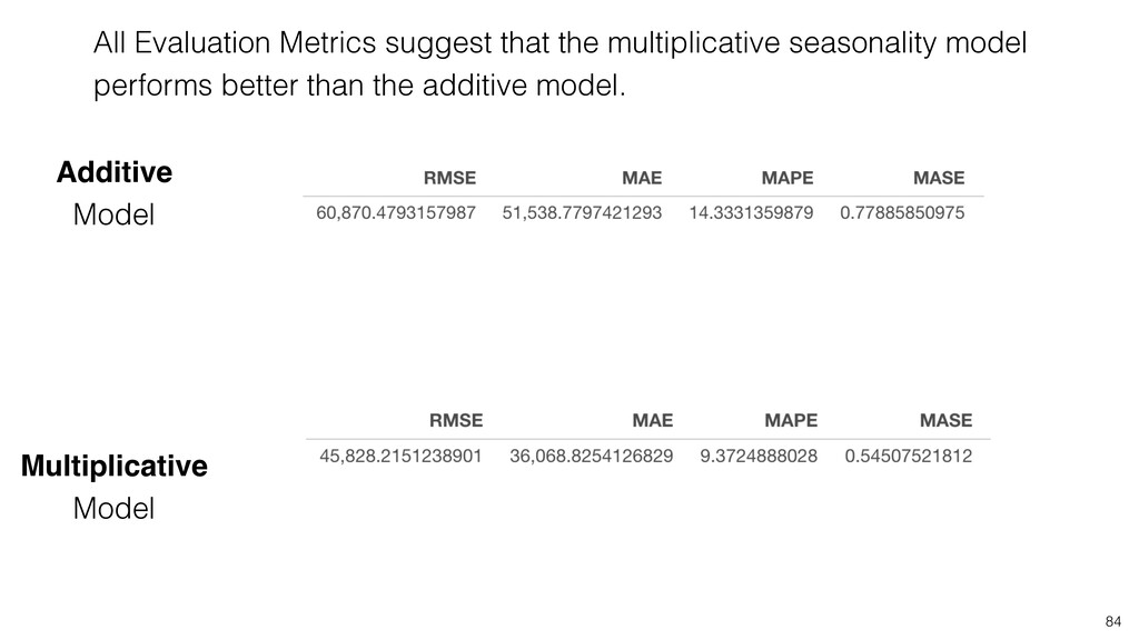
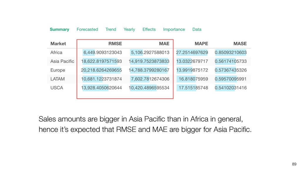
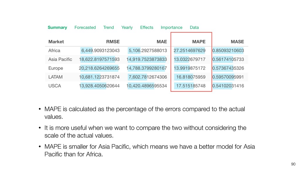
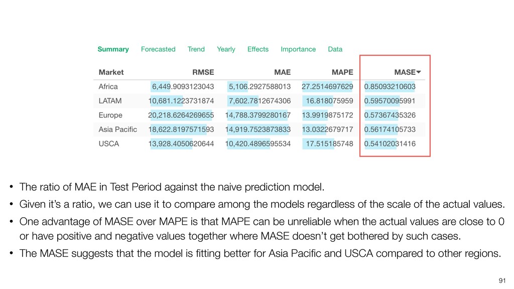
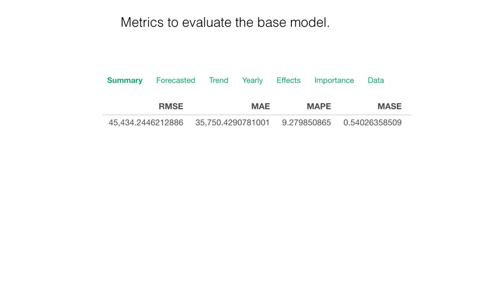
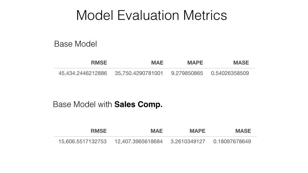
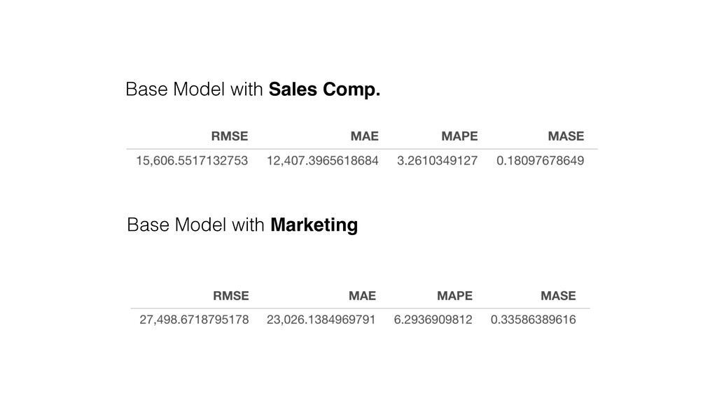
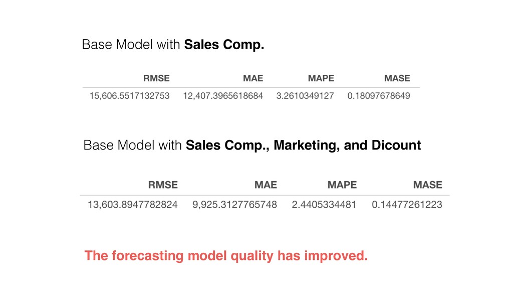
57. • MAE (Mean Absolute Error) : Mean of absolute differences between actual value and forecasted value. • RMSE (Root Mean Square Error) : Root of mean of squares of difference between actual value and forecasted value. • MAPE (Mean Absolute Percentage Error) : Mean of absolute differences in percentage of actual value. • MASE (Mean Absolute Scaled Error) : Divide MAE of the forecasting model by MAE of a naive forecasting model (a simple model that always forecasts one previous value). Metrics to Evaluate Forecasting Model
58. Root
 Mean
 Square
 Error Square the Errors (Difference between the actual and the forecasted), take the mean, and root the mean. 58 RMSE (Root Mean Square Error)
59. 
 22 + 22 + 22 + 42 
 4 4 + 4 + 4 + 16 
 4 7 = 2.65 59 RMSE (Root Mean Square Error) 2 2 4 2 = =
60. Mean
 Absolute
 Error Absolute values of the Errors (Difference between the actual and the forecasted) and take the mean. 60 MAE (Mean Absolute Error)
61. 
 2 + 2 + 2 + 4 
 4 61 = 2.5 MAE (Mean Absolute Error) 2 2 4 2
62. Mean
 Absolute
 Percentage
 Error Absolute Percentage differences between the actual and the forecasted and take the mean. 62 MAPE (Mean Absolute Percentage Error)
63. 63 12 13 16 11 Take the actual values. MAPE (Mean Absolute Percentage Error)
64. 64 12 13 16 11 MAPE (Mean Absolute Percentage Error) 2 2 4 2 Take the errors.
65. 65 100 100 100 100 MAPE (Mean Absolute Percentage Error) 16.6% 15.4% 25% 18.2% Calculate the ratio of the errors against the actual values. If it’s negative make it positive. (Absolute)
66. 66 100 100 100 100 MAPE (Mean Absolute Percentage Error) 16.6% 15.4% 25% 18.2% 
 16.6 + 15.4 + 18.2 + 25 
 4 Take the mean. = 18.8%
67. 67 Mean
 Absolute
 Scaled
 Error Scale the MAE so that it can be compared among data sets with different variability. MASE (Mean Absolute Scaled Error)
68. 68 MAE in the test period / MAE of a ‘naive’ prediction model in the training period MASE - How to Scale
69. 69 Use the Previous Period Values as the Forecasted Values Naive Forecasting
70. 70 MAE in Training Period
71. 71 MAE in the test period MAE of a ‘naive’ prediction model in the training period MASE = MAE in the test period / MAE of a ‘naive’ prediction model in the training period
72. 72 Seasonality Mode Additive vs. Multiplicative
73. 73 The difference between the actual line and the forecasted line becomes wider as the time progresses.
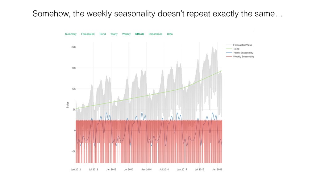
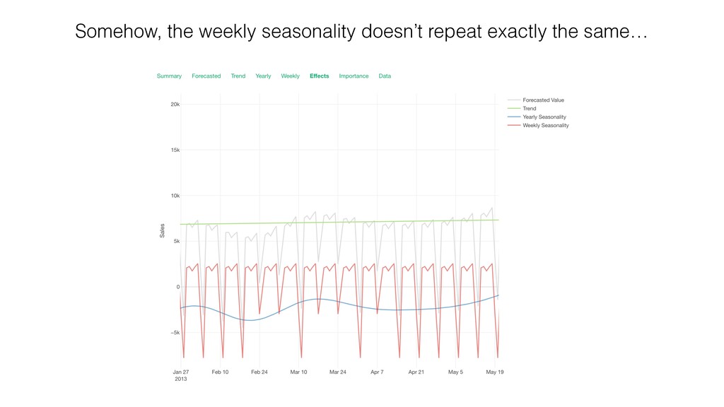
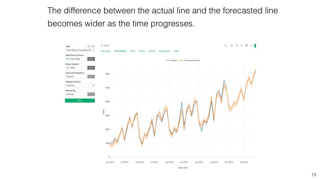
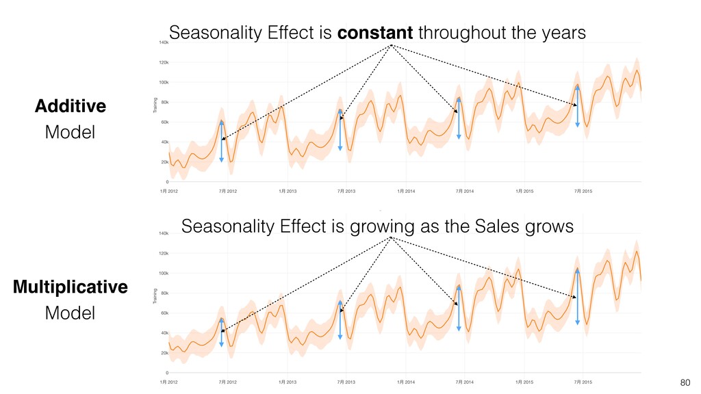
74. What’s happening? 74 • This model is assuming that the seasonal variability stays the constant. • But, as Sales increases maybe the seasonal variability increases, too. • This model might not be able to keep up with the actual growth of Sales. Can we model the seasonality that also grows as the Sales grows?
75. Additive Growth Multiplicative Growth Number of Employees at a very stable company Amazon’s Sales Trend Different Types of Growth Models 75
76. 76 The effect is additive The effect is multiplicative Additive Multiplicative Seasonality Mode Grows 20% in February Grows $20,000 in February The growth is constant regardless of the previous value The growth rate is constant, which means it grows bigger when the previous value big.
77. Switch Seasonality Mode to ‘Multiplicative’ 77
78. The difference between the actual and the forecasted looks similar even as the time progresses.
79. 79 Additive Model Multiplicative Model
80. 80 Seasonality Effect is constant throughout the years Seasonality Effect is growing as the Sales grows Additive Model Multiplicative Model
81. 81 Additive Model Multiplicative Model Seasonality Effect is constant throughout the years Seasonality Effect is growing as the Sales grows
82. 82 Building Forecasting Models for Monthly Sales Additive Model Multiplicative Model
83. 83 The Additive Seasonality model is not keeping up with the actual Sales growth while the Multiplicative model is performing better. Additive Model Multiplicative Model
84. 84 Additive Model Multiplicative Model All Evaluation Metrics suggest that the multiplicative seasonality model performs better than the additive model.
85. Compare the Models among Markets with Repeat By
86. 86 To compare among Markets, select ‘Market’ for Repeat By and build multiple forecasting models.
88. • RMSE and MAE indicate that the errors are smaller for Africa compared to Asia Pacific. • Can we conclude that the model for Africa is better? 88
89. 89 Sales amounts are bigger in Asia Pacific than in Africa in general, hence it’s expected that RMSE and MAE are bigger for Asia Pacific.
90. • MAPE is calculated as the percentage of the errors compared to the actual values. • It is more useful when we want to compare the two without considering the scale of the actual values. • MAPE is smaller for Asia Pacific, which means we have a better model for Asia Pacific than for Africa. 90
91. 91 • The ratio of MAE in Test Period against the naive prediction model. • Given it’s a ratio, we can use it to compare among the models regardless of the scale of the actual values. • One advantage of MASE over MAPE is that MAPE can be unreliable when the actual values are close to 0 or have positive and negative values together where MASE doesn’t get bothered by such cases. • The MASE suggests that the model is fitting better for Asia Pacific and USCA compared to other regions.
92. External Predictors
93. If we know some variables are correlated with Sales and we can get to know the future values of such variables, can’t we forecast better?
94. Sales and Sales Comp. look correlated to one another.
95. Sales and Marketing look correlated to one another, too.
96. Sales and Discount (Avg) don’t look correlated to one another.
97. Marketing Let’s say we can control how much we will be spending on the marketing in the next 3 months. Can we make such information built into the forecasting model? Example
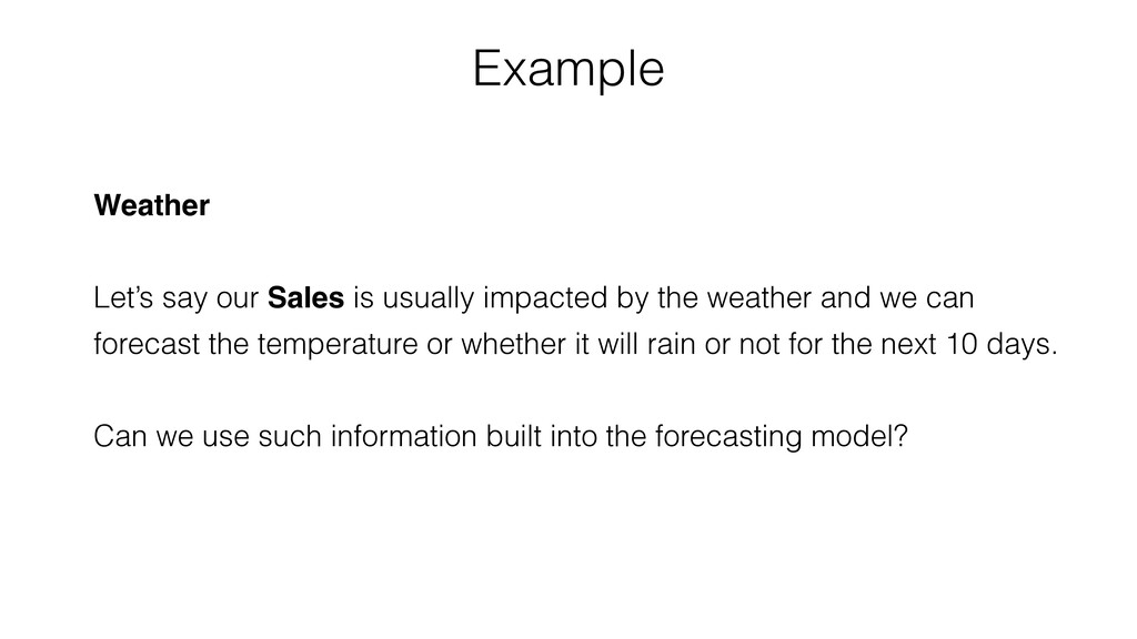
98. Weather Let’s say our Sales is usually impacted by the weather and we can forecast the temperature or whether it will rain or not for the next 10 days. Can we use such information built into the forecasting model? Example
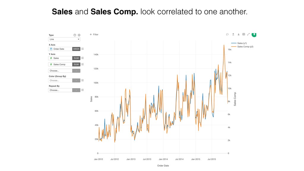
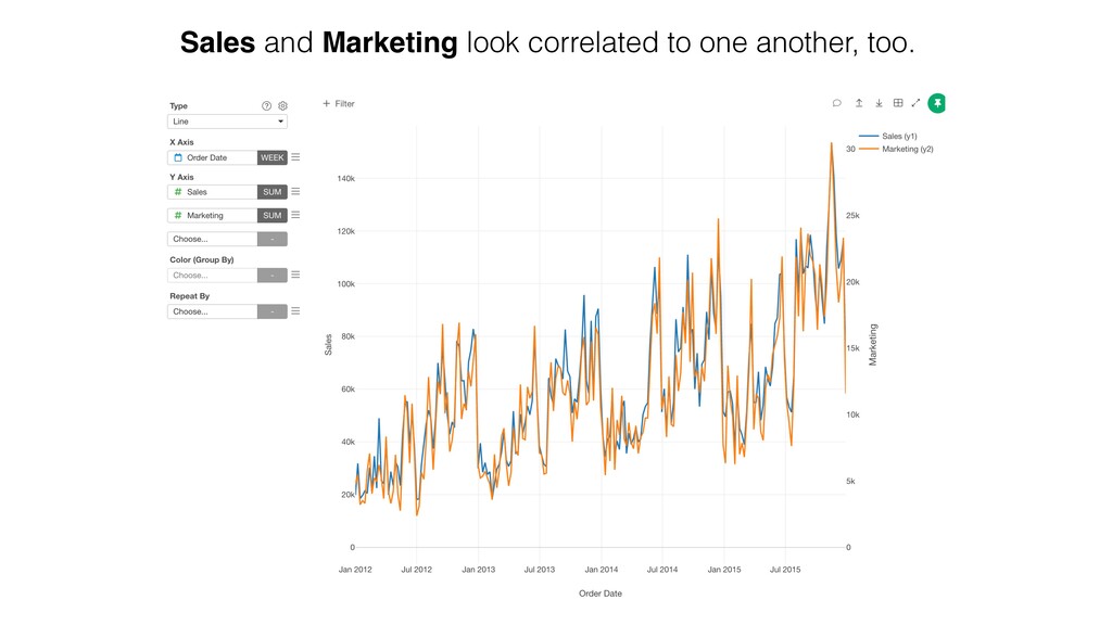
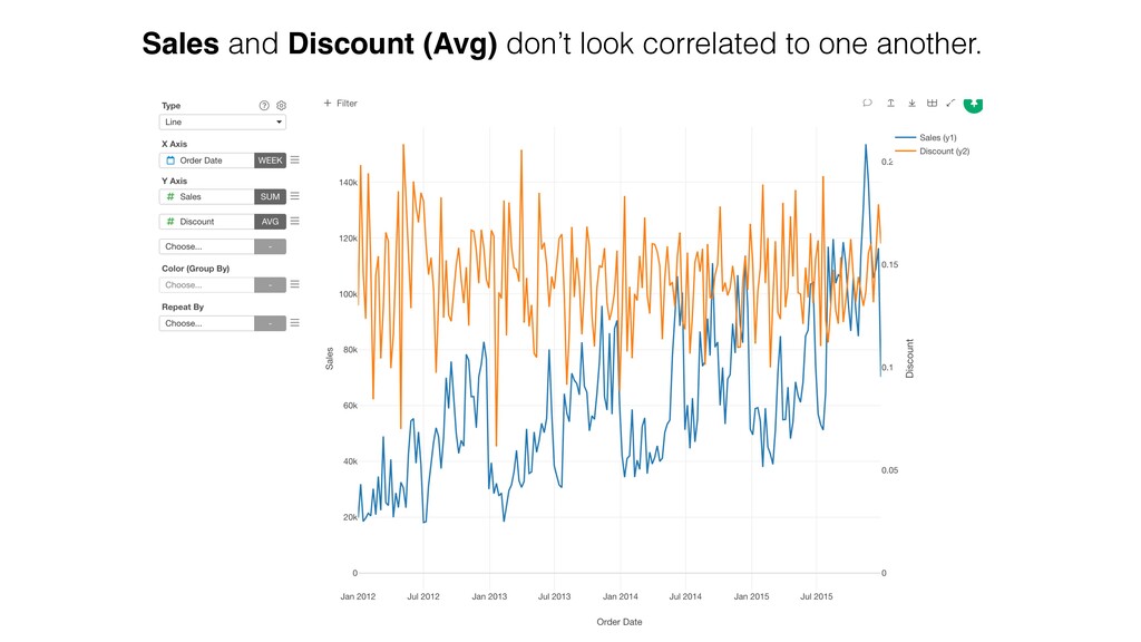
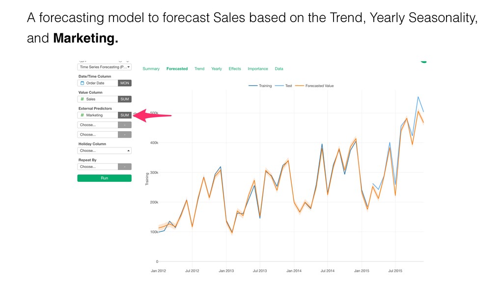
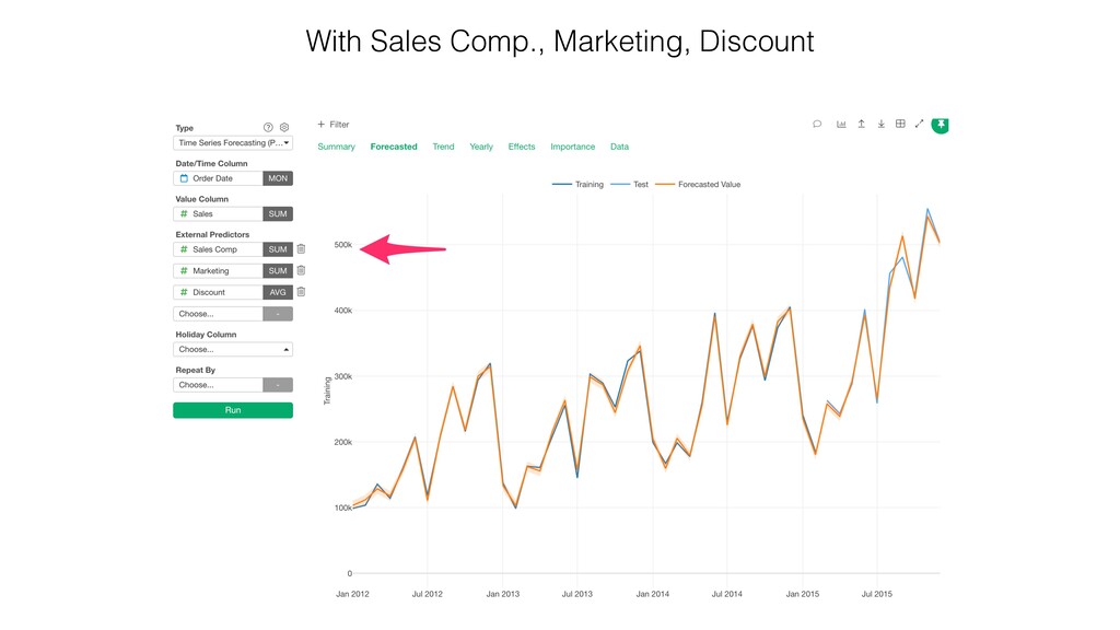
99. You can assign variables as ‘External Predictors (Extra Regressors) and build forecasting models. Prophet investigate if the external predictor (Marketing) is useful to build a better model forecast the target variable (Sales) and calculate the coefficient of the predictor variable. External Predictors
100. A forecasting model to forecast Sales based on the Trend, Yearly Seasonality with Test Mode.
101. Metrics to evaluate the base model.
102. A forecasting model to forecast Sales based on the Trend, Yearly Seasonality, and Sales Comp.
103. Model Evaluation Metrics Base Model Base Model with Sales Comp.
104. A forecasting model to forecast Sales based on the Trend, Yearly Seasonality, and Marketing.
105. Base Model with Sales Comp. Base Model with Marketing
106. How about all of them together? Sales Comp., Marketing, and Discount
107. With Sales Comp., Marketing, Discount
108. Base Model with Sales Comp. Base Model with Sales Comp., Marketing, and Dicount The forecasting model quality has improved.
109. Under the Effects tab, you can see how each of the seasonality and the predictor variables are effecting on the forecasted values.
110. Under the Importance tab, you can comparesee how each of the seasonality and the predictor variables are effecting on the forecasted values.
111. Advanced Topics
112. Holiday Effect
113. 113 • Holiday might effect the measures like sales, number of orders, etc. • Special events like conferences, black friday, sports events, etc. might effect the measures. Holiday Effect
114. 114 Unique Page Views of ”Apple Worldwide Developers Conference” (WWDC) at Wikipedia Data
115. 115 Apple Worldwide Developers Conference (WWDC) dates Data
116. 116 Data Future dates.
117. • Set ‘Day’ for Date / Time • Set 365 as Forecasting Time Period Forecast without Considering Holiday Effect 117
118. 118 These WWDC dates are not forecasted well by the model.
119. Add WWDC Dates by Join
120. Select ‘Full join’ as the join type because we want to bring the dates that don’t exist in the current data frame but does exist in the target data frame. Add WWDC Dates by Join 120
122. Select Holiday Column 122 These WWDC dates are not forecasted well by the model.
123. 123 Future conference dates are better forecasted by incorporating the holiday effect.
124. 124 Holidays Tab Green line is the Holiday effect.
126. Capacity
127. 127 Capacity - Upper / Lower Limit
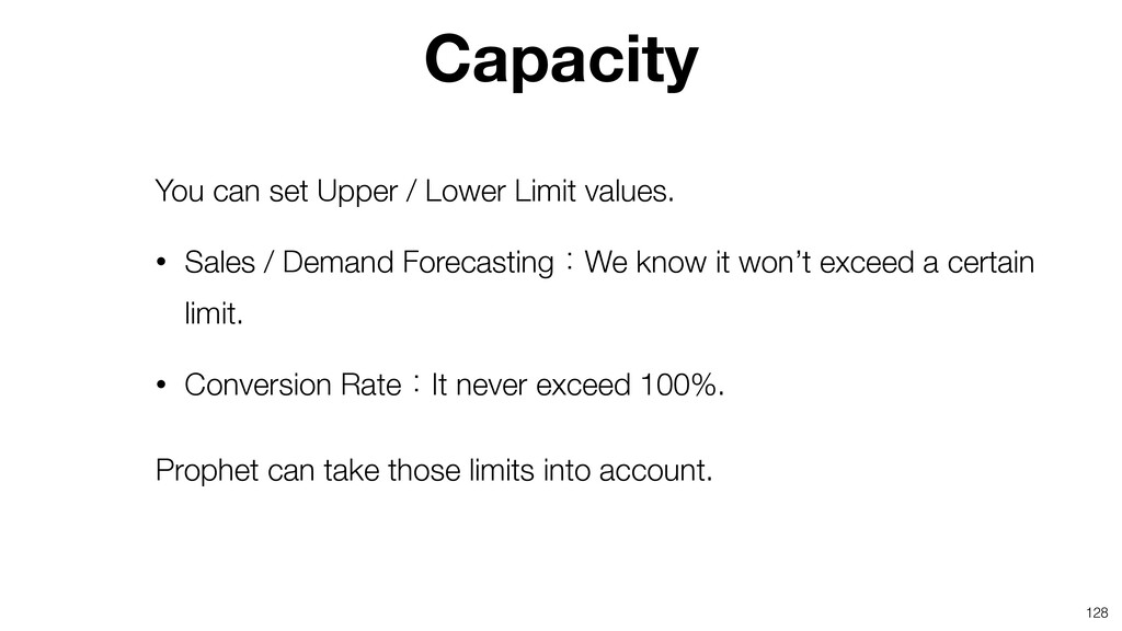
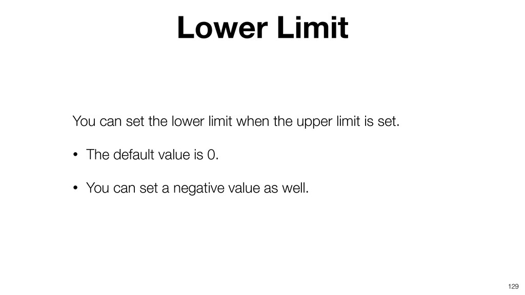
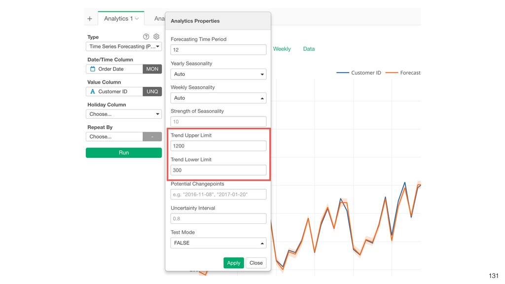
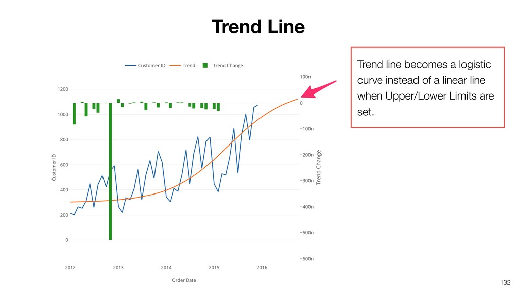
128. 128 You can set Upper / Lower Limit values. • Sales / Demand ForecastingɿWe know it won’t exceed a certain limit. • Conversion RateɿIt never exceed 100%. Prophet can take those limits into account. Capacity
129. 129 You can set the lower limit when the upper limit is set. • The default value is 0. • You can set a negative value as well. Lower Limit
132. Trend Line 132 Trend line becomes a logistic curve instead of a linear line when Upper/Lower Limits are set.
133. Q & A
134. Information Email kan@exploratory.io Website https://exploratory.io Twitter @KanAugust Training https://exploratory.io/training
135. EXPLORATORY