Survey on DANN

Transcript

1. Domain Adversarial Training of Neural Networks [Ganin+ JMLR 2016] Kenshin Abe 2020/05/20 1
2. Paper Introduction 2
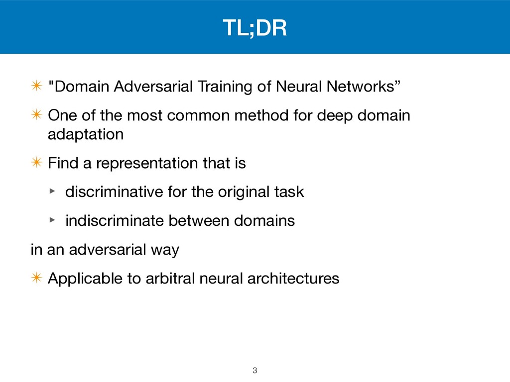
3. TL;DR ✴ "Domain Adversarial Training of Neural Networks” ✴ One of the most common method for deep domain adaptation ✴ Find a representation that is ‣ discriminative for the original task ‣ indiscriminate between domains in an adversarial way ✴ Applicable to arbitral neural architectures 3
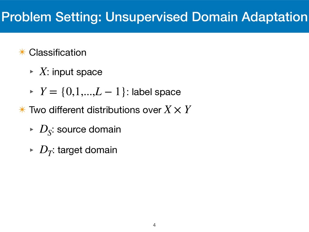
4. Problem Setting: Unsupervised Domain Adaptation ✴ Classification ‣ : input space ‣ : label space ✴ Two different distributions over ‣ : source domain ‣ : target domain X Y = {0,1,...,L − 1} X × Y DS DT 4
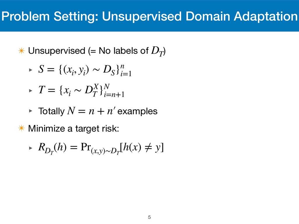
5. Problem Setting: Unsupervised Domain Adaptation ✴ Unsupervised (= No labels of ) ‣ ‣ ‣ Totally examples ✴ Minimize a target risk: ‣ DT S = {(xi , yi ) ∼ DS }n i=1 T = {xi ∼ DX T }N i=n+1 N = n + n′ RDT (h) = Pr(x,y)∼DT [h(x) ≠ y] 5
6. Background Theory 6
7. H-divergence [Ben-David+ NIPS 2006] ✴ Discrepancy measure ✴ Given and over , and a hypothesis class , ‣ “How distinguishable two classes are by ” ✴ Empirical H-divergence DX S DX T X H dH (DX S , DX T ) = 2 sup h∈H |Prx∼DX S [h(x) = 1] − Prx∼DX T [h(x) = 1]| H ˜ dH (S, H) = 2(1 − min h∈H ( 1 n n ∑ i=1 I[h(xi ) = 0] + 1 n′ N ∑ i=n+1 I[h(xi ) = 1])) 7
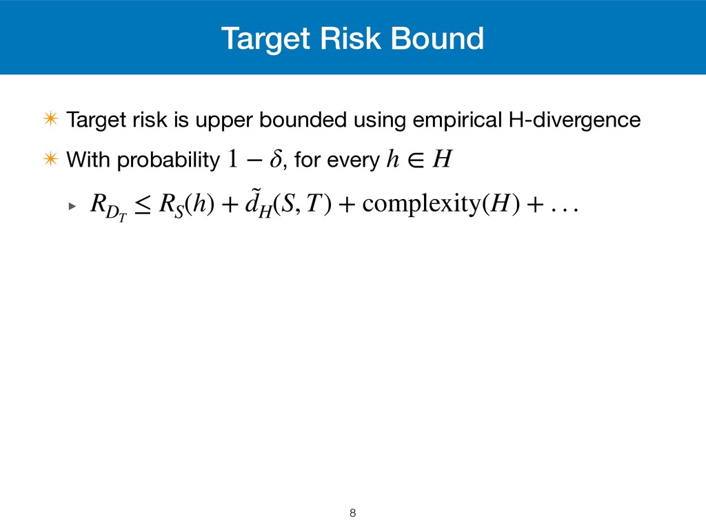
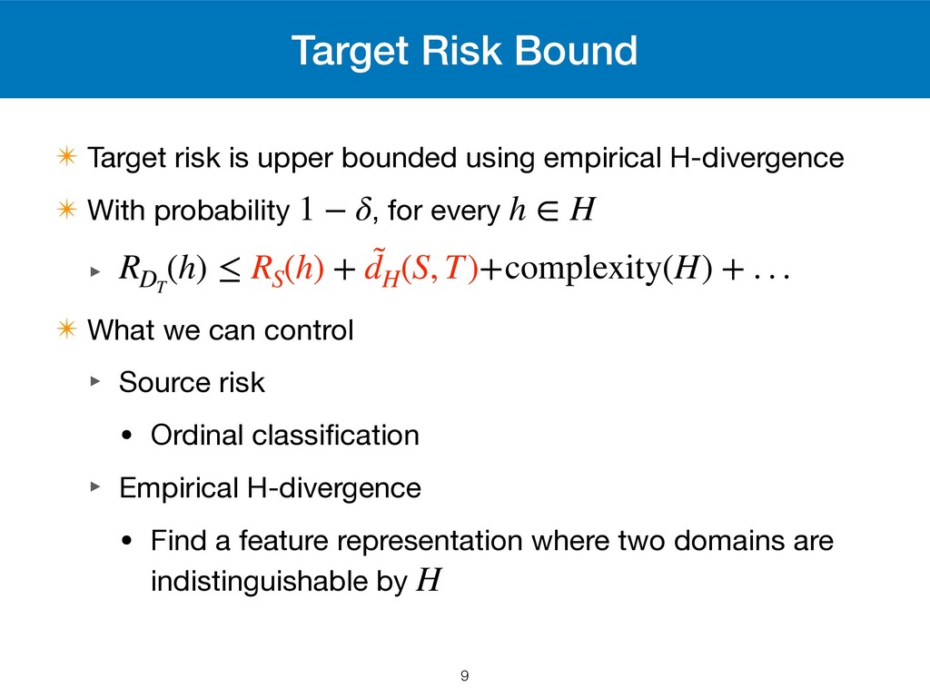
8. Target Risk Bound ✴ Target risk is upper bounded using empirical H-divergence ✴ With probability , for every ‣ 1 − δ h ∈ H RDT ≤ RS (h) + ˜ dH (S, T) + complexity(H) + . . . 8
9. Target Risk Bound ✴ Target risk is upper bounded using empirical H-divergence ✴ With probability , for every ‣ ✴ What we can control ‣ Source risk • Ordinal classification ‣ Empirical H-divergence • Find a feature representation where two domains are indistinguishable by 1 − δ h ∈ H RDT (h) ≤ RS (h) + ˜ dH (S, T)+complexity(H) + . . . H 9
10. Architecture 10
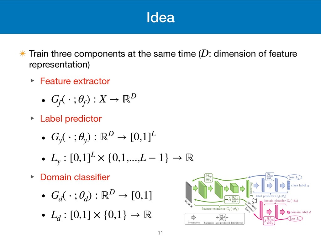
11. Idea ✴ Train three components at the same time ( : dimension of feature representation) ‣ Feature extractor • ‣ Label predictor • • ‣ Domain classifier • • D Gf ( ⋅ ; θf ) : X → ℝD Gy ( ⋅ ; θy ) : ℝD → [0,1]L Ly : [0,1]L × {0,1,...,L − 1} → ℝ Gd ( ⋅ ; θd ) : ℝD → [0,1] Ld : [0,1] × {0,1} → ℝ 11
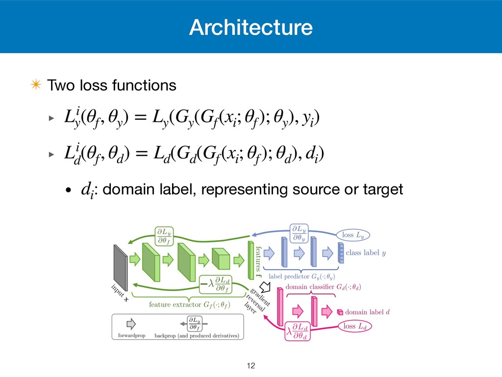
12. Architecture ✴ Two loss functions ‣ ‣ • : domain label, representing source or target Li y (θf , θy ) = Ly (Gy (Gf (xi ; θf ); θy ), yi ) Li d (θf , θd ) = Ld (Gd (Gf (xi ; θf ); θd ), di ) di 12
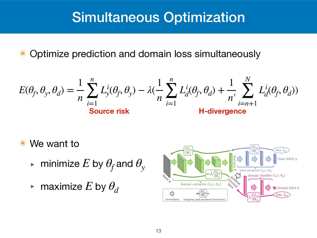
13. Simultaneous Optimization ✴ Optimize prediction and domain loss simultaneously ✴ We want to ‣ minimize by and ‣ maximize by E(θf , θy , θd ) = 1 n n ∑ i=1 Li y (θf , θy ) − λ( 1 n n ∑ i=1 Li d (θf , θd ) + 1 n′ N ∑ i=n+1 Li d (θf , θd )) E θf θy E θd 13 Source risk H-divergence
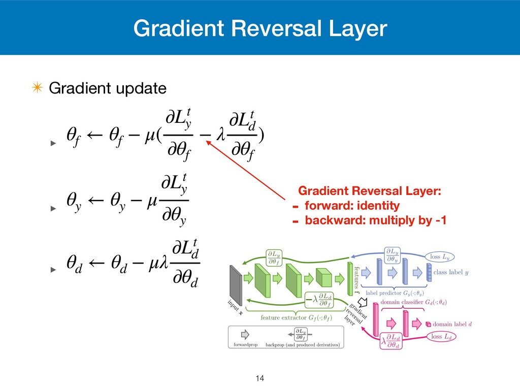
14. Gradient Reversal Layer ✴ Gradient update ‣ ‣ ‣ θf ← θf − μ( ∂Lt y ∂θf − λ ∂Lt d ∂θf ) θy ← θy − μ ∂Lt y ∂θy θd ← θd − μλ ∂Lt d ∂θd 14 Gradient Reversal Layer: - forward: identity - backward: multiply by -1
15. Summary 15
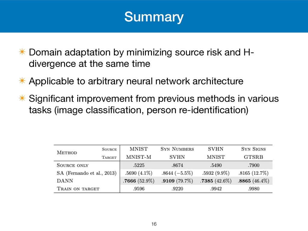
16. Summary ✴ Domain adaptation by minimizing source risk and H- divergence at the same time ✴ Applicable to arbitrary neural network architecture ✴ Significant improvement from previous methods in various tasks (image classification, person re-identification) 16