Policy Preference Affected by Perceived Fact on Externality: Why Do People with Higher Socio‐economic Status Sometimes Prefer Stronger Income Equalization Policy?
Presentation at the 19th ISA World Congress of Sociology, Toronto, Canada, July 18, 2018
People with Higher Socio‐economic Status Sometimes Prefer Stronger Income Equalization Policy? Koji YAMAMOTO (Hylab LLP and the Open University of Japan) Presentation at the 19th ISA World Congress of Sociology, Toronto, Canada, July 18, 2018
– Literature: Higher SES Against redistribution – Background question: How could people come close to agreement, instead of conflict, over public policy? 4
look at “whole picture” of society “Be‐the‐Government” – Sources of preference: • Normative evaluation criteria • Perceived fact (information on reality) 5
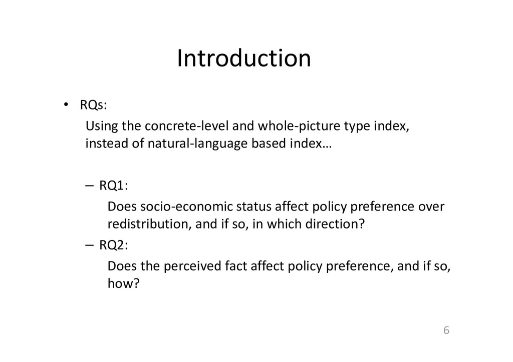
instead of natural‐language based index… – RQ1: Does socio‐economic status affect policy preference over redistribution, and if so, in which direction? – RQ2: Does the perceived fact affect policy preference, and if so, how? 6
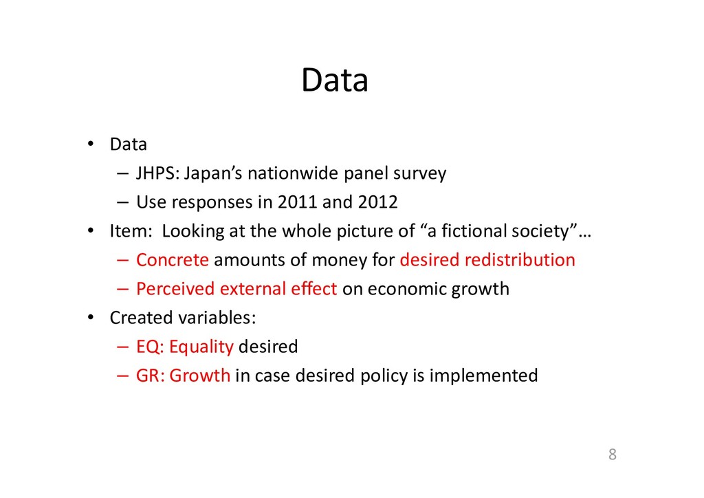
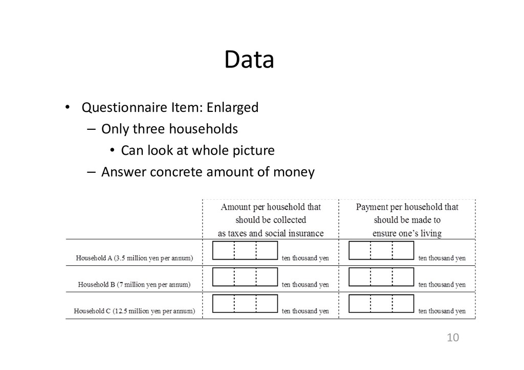
Use responses in 2011 and 2012 • Item: Looking at the whole picture of “a fictional society”… – Concrete amounts of money for desired redistribution – Perceived external effect on economic growth • Created variables: – EQ: Equality desired – GR: Growth in case desired policy is implemented 8
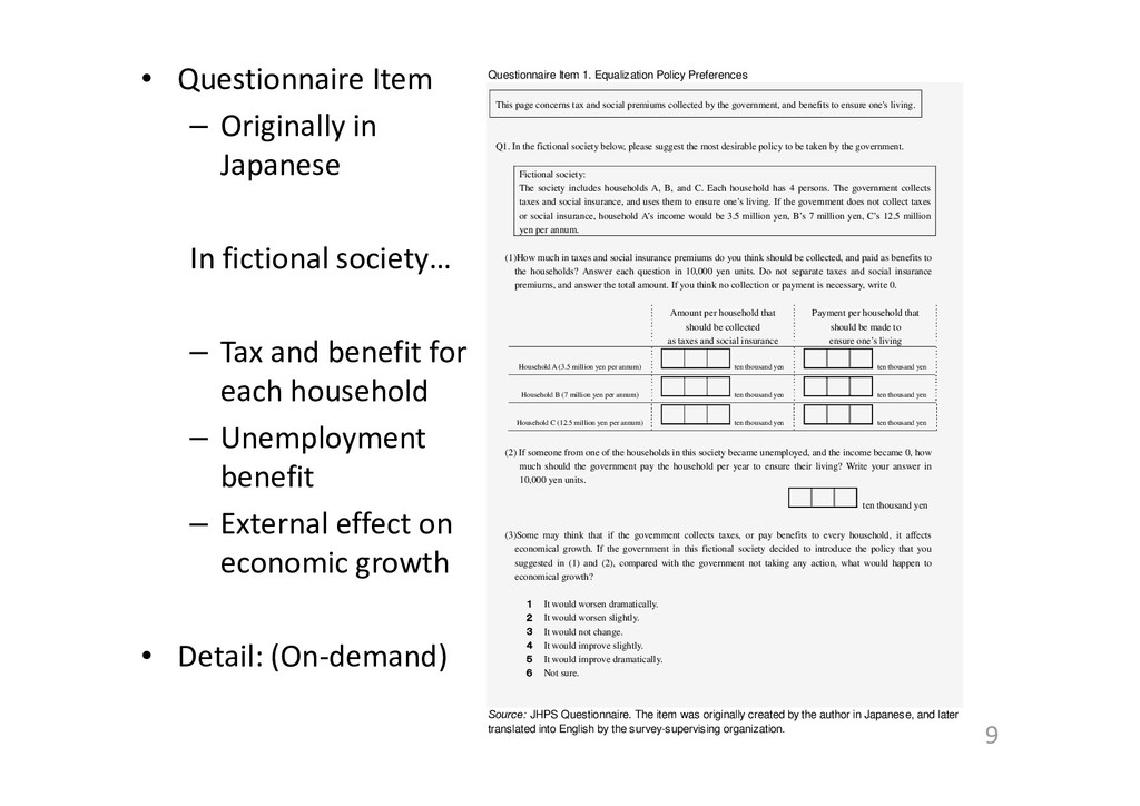
– Tax and benefit for each household – Unemployment benefit – External effect on economic growth • Detail: (On‐demand) 9 Questionnaire Item 1. Equalization Policy Preferences Source: JHPS Questionnaire. The item was originally created by the author in Japanese, and later translated into English by the survey-supervising organization. This page concerns tax and social premiums collected by the government, and benefits to ensure one's living. Q1. In the fictional society below, please suggest the most desirable policy to be taken by the government. Fictional society: The society includes households A, B, and C. Each household has 4 persons. The government collects taxes and social insurance, and uses them to ensure one’s living. If the government does not collect taxes or social insurance, household A’s income would be 3.5 million yen, B’s 7 million yen, C’s 12.5 million yen per annum. (1)How much in taxes and social insurance premiums do you think should be collected, and paid as benefits to the households? Answer each question in 10,000 yen units. Do not separate taxes and social insurance premiums, and answer the total amount. If you think no collection or payment is necessary, write 0. Amount per household that should be collected as taxes and social insurance Payment per household that should be made to ensure one’s living Household A (3.5 million yen per annum) ten thousand yen ten thousand yen Household B (7 million yen per annum) ten thousand yen ten thousand yen Household C (12.5 million yen per annum) ten thousand yen ten thousand yen (2) If someone from one of the households in this society became unemployed, and the income became 0, how much should the government pay the household per year to ensure their living? Write your answer in 10,000 yen units. ten thousand yen (3)Some may think that if the government collects taxes, or pay benefits to every household, it affects economical growth. If the government in this fictional society decided to introduce the policy that you suggested in (1) and (2), compared with the government not taking any action, what would happen to economical growth? 1 It would worsen dramatically. 2 It would worsen slightly. 3 It would not change. 4 It would improve slightly. 5 It would improve dramatically. 6 Not sure.
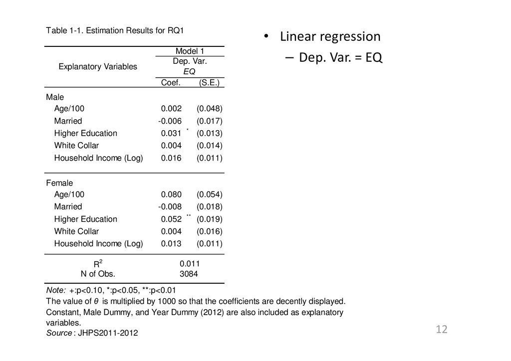
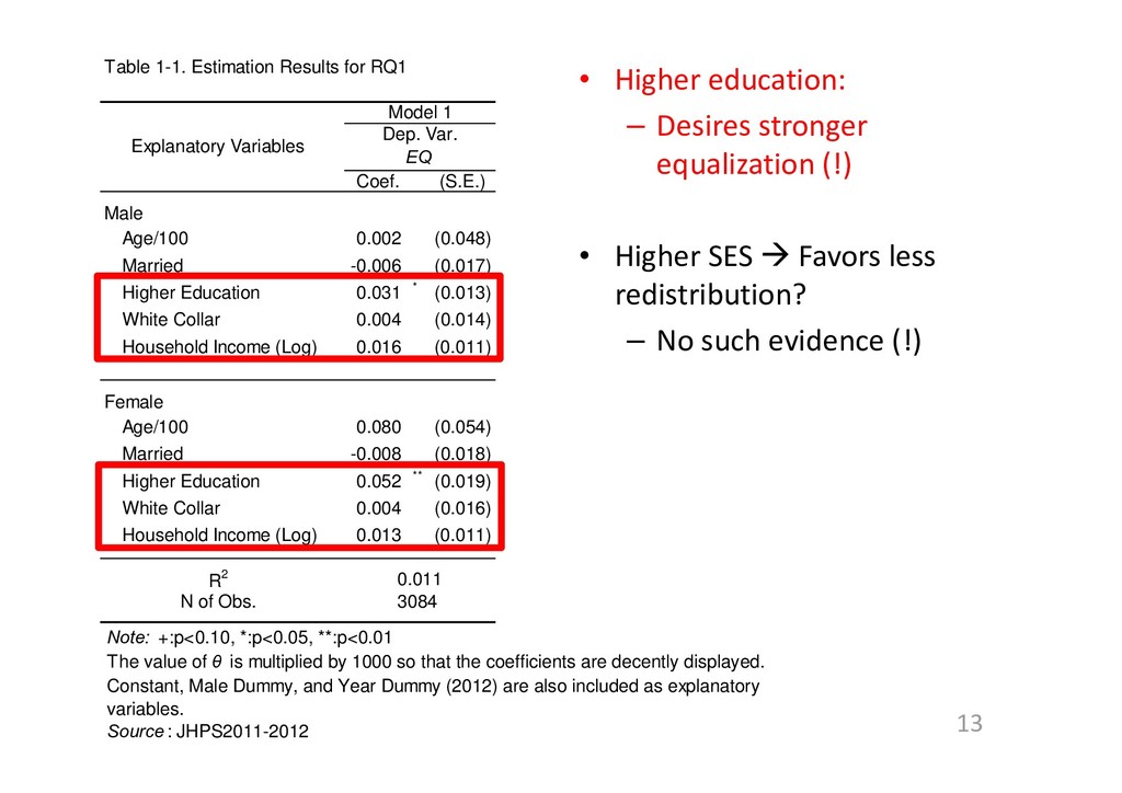
: JHPS2011-2012 Note: +:p<0.10, *:p<0.05, **:p<0.01 The value of θ is multiplied by 1000 so that the coefficients are decently displayed. Constant, Male Dummy, and Year Dummy (2012) are also included as explanatory variables. Table 1-1. Estimation Results for RQ1 Coef. (S.E.) Male Age/100 0.002 (0.048) Married -0.006 (0.017) Higher Education 0.031 * (0.013) White Collar 0.004 (0.014) Household Income (Log) 0.016 (0.011) Female Age/100 0.080 (0.054) Married -0.008 (0.018) Higher Education 0.052 ** (0.019) White Collar 0.004 (0.016) Household Income (Log) 0.013 (0.011) N of Obs. 3084 R2 0.011 Explanatory Variables Model 1 Dep. Var. EQ
SES Favors less redistribution? – No such evidence (!) 13 Source : JHPS2011-2012 Note: +:p<0.10, *:p<0.05, **:p<0.01 The value of θ is multiplied by 1000 so that the coefficients are decently displayed. Constant, Male Dummy, and Year Dummy (2012) are also included as explanatory variables. Table 1-1. Estimation Results for RQ1 Coef. (S.E.) Male Age/100 0.002 (0.048) Married -0.006 (0.017) Higher Education 0.031 * (0.013) White Collar 0.004 (0.014) Household Income (Log) 0.016 (0.011) Female Age/100 0.080 (0.054) Married -0.008 (0.018) Higher Education 0.052 ** (0.019) White Collar 0.004 (0.016) Household Income (Log) 0.013 (0.011) N of Obs. 3084 R2 0.011 Explanatory Variables Model 1 Dep. Var. EQ
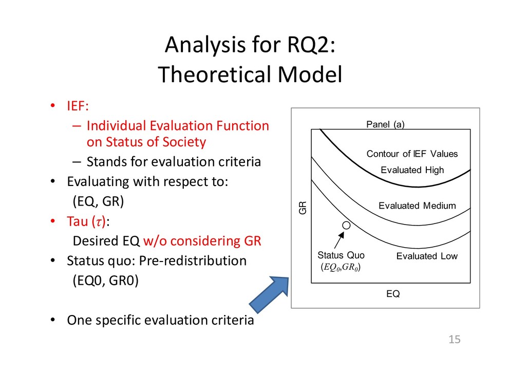
Function on Status of Society – Stands for evaluation criteria • Evaluating with respect to: (EQ, GR) • Tau (τ): Desired EQ w/o considering GR • Status quo: Pre‐redistribution (EQ0, GR0) • One specific evaluation criteria 15 GR EQ Panel (a) Status Quo (EQ0 ,GR0 ) Contour of IEF Values Evaluated High Evaluated Medium Evaluated Low
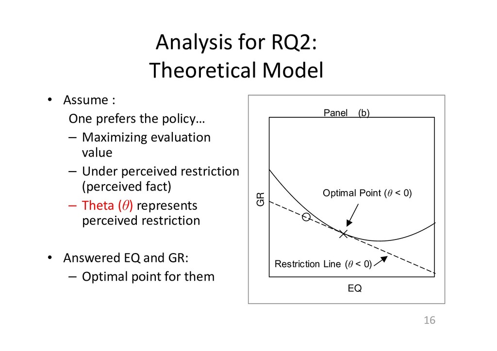
the policy… – Maximizing evaluation value – Under perceived restriction (perceived fact) – Theta (θ) represents perceived restriction • Answered EQ and GR: – Optimal point for them 16 GR EQ Panel (b) Restriction Line (θ < 0) Optimal Point (θ < 0)
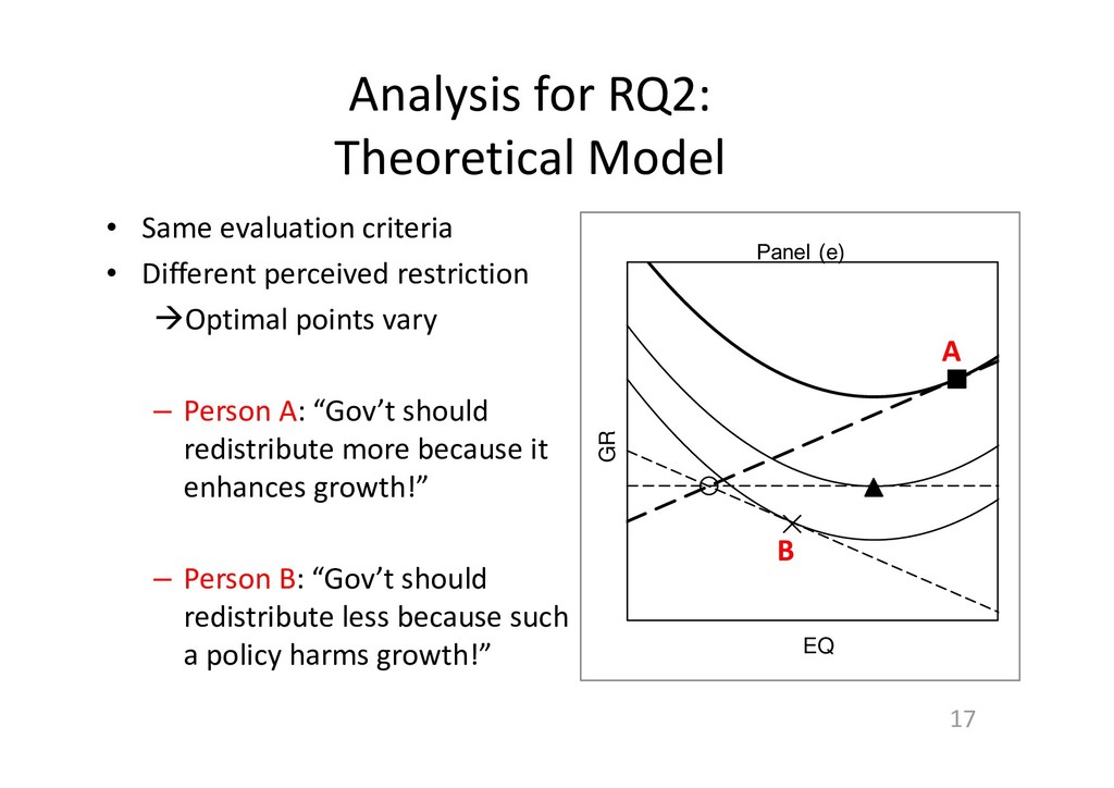
Different perceived restriction Optimal points vary – Person A: “Gov’t should redistribute more because it enhances growth!” – Person B: “Gov’t should redistribute less because such a policy harms growth!” 17 GR EQ Panel (e) A B
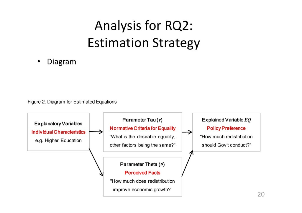
Diagram for Estimated Equations Explained Variable EQ Policy Preference "How much redistribution should Gov't conduct?" Parameter Theta (θ) Perceived Facts "How much does redistribution improve economic growth?" Parameter Tau (τ) Normative Criteria for Equality "What is the desirable equality, other factors being the same?" Explanatory Variables Individual Characteristics e.g. Higher Education
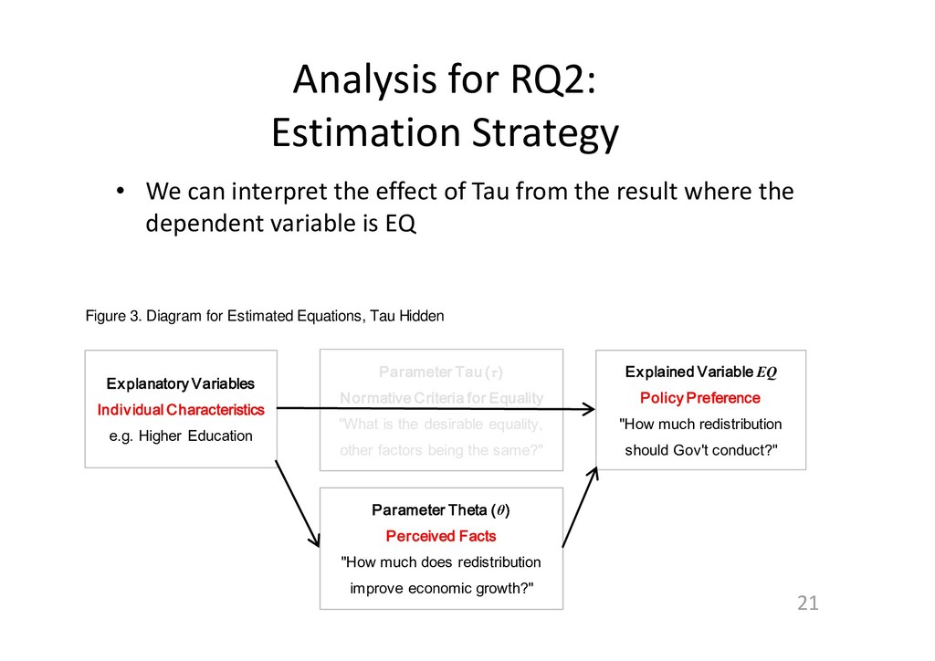
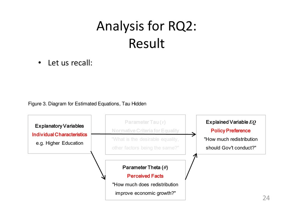
effect of Tau from the result where the dependent variable is EQ 21 Figure 3. Diagram for Estimated Equations, Tau Hidden Explained Variable EQ Policy Preference "How much redistribution should Gov't conduct?" Parameter Theta (θ) Perceived Facts "How much does redistribution improve economic growth?" Parameter Tau (τ) Normative Criteria for Equality "What is the desirable equality, other factors being the same?" Explanatory Variables Individual Characteristics e.g. Higher Education
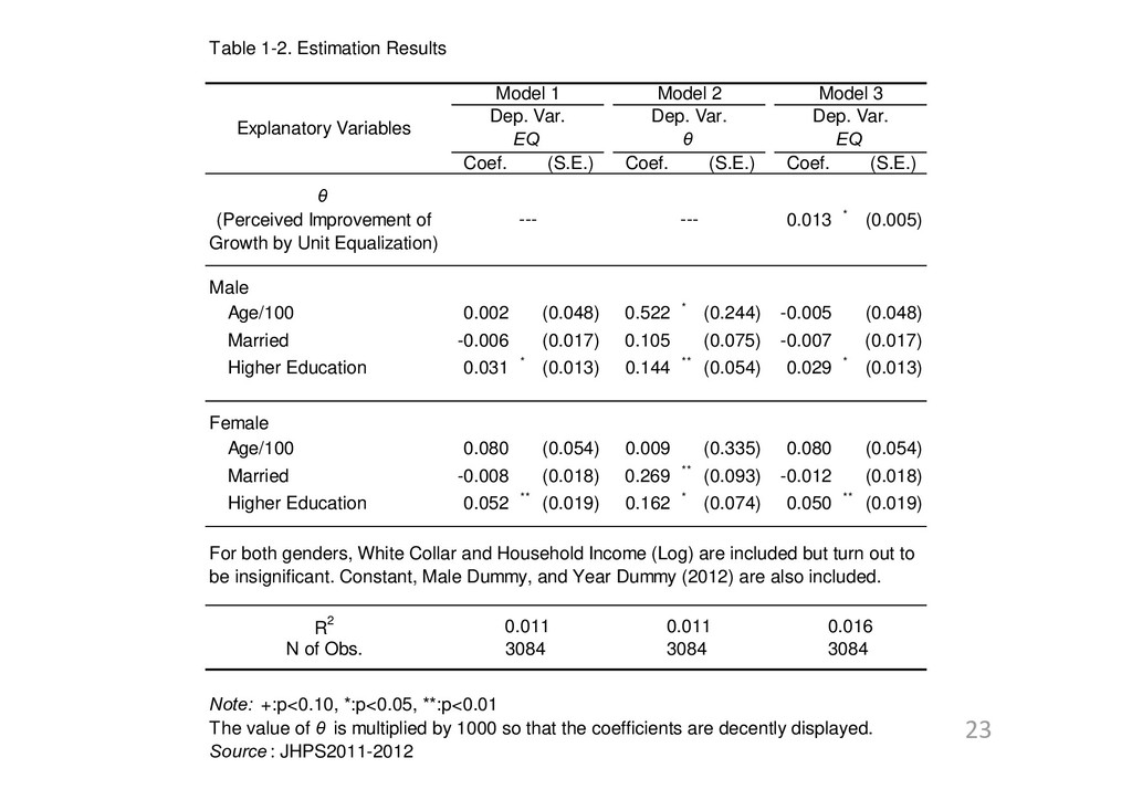
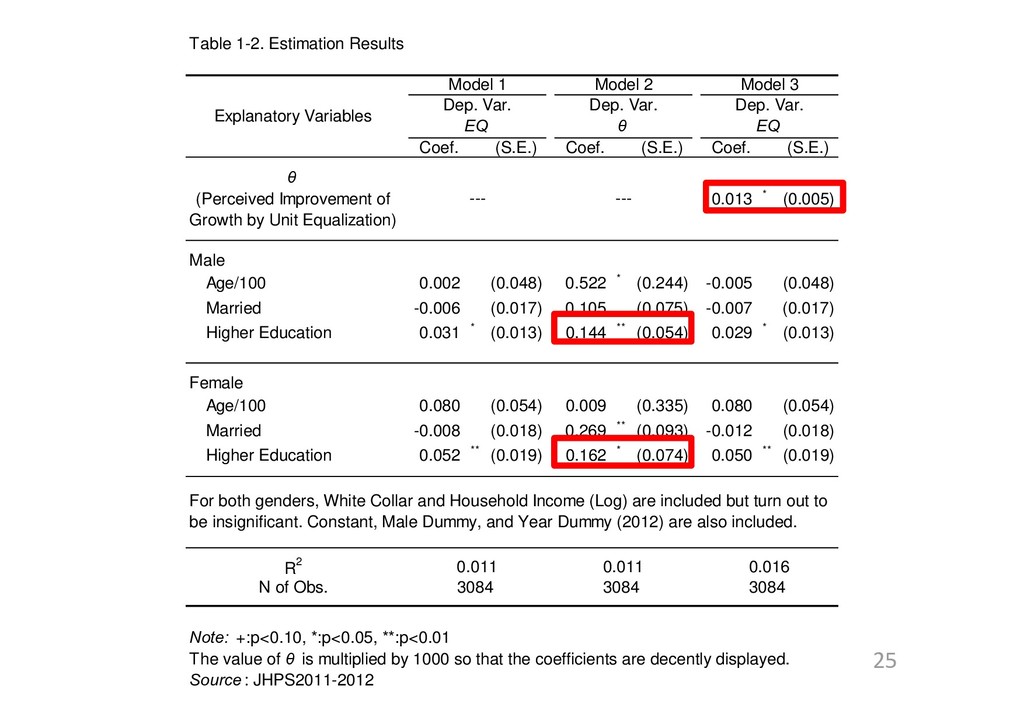
(S.E.) 0.013 * (0.005) Male Age/100 0.002 (0.048) 0.522 * (0.244) -0.005 (0.048) Married -0.006 (0.017) 0.105 (0.075) -0.007 (0.017) Higher Education 0.031 * (0.013) 0.144 ** (0.054) 0.029 * (0.013) Female Age/100 0.080 (0.054) 0.009 (0.335) 0.080 (0.054) Married -0.008 (0.018) 0.269 ** (0.093) -0.012 (0.018) Higher Education 0.052 ** (0.019) 0.162 * (0.074) 0.050 ** (0.019) Source : JHPS2011-2012 Note: +:p<0.10, *:p<0.05, **:p<0.01 The value of θ is multiplied by 1000 so that the coefficients are decently displayed. θ (Perceived Improvement of Growth by Unit Equalization) --- --- R2 0.011 0.011 For both genders, White Collar and Household Income (Log) are included but turn out to be insignificant. Constant, Male Dummy, and Year Dummy (2012) are also included. 0.016 N of Obs. 3084 3084 3084 Explanatory Variables Model 1 Model 2 Model 3 Dep. Var. Dep. Var. Dep. Var. EQ θ EQ
3. Diagram for Estimated Equations, Tau Hidden Explained Variable EQ Policy Preference "How much redistribution should Gov't conduct?" Parameter Theta (θ) Perceived Facts "How much does redistribution improve economic growth?" Parameter Tau (τ) Normative Criteria for Equality "What is the desirable equality, other factors being the same?" Explanatory Variables Individual Characteristics e.g. Higher Education
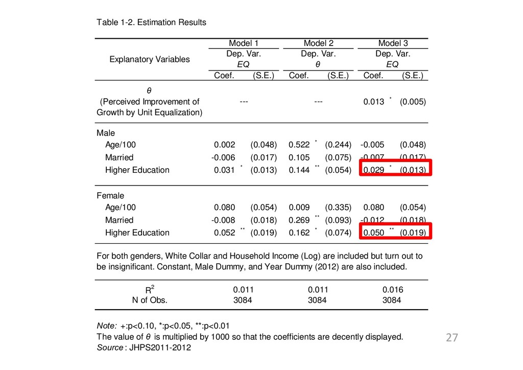
(S.E.) 0.013 * (0.005) Male Age/100 0.002 (0.048) 0.522 * (0.244) -0.005 (0.048) Married -0.006 (0.017) 0.105 (0.075) -0.007 (0.017) Higher Education 0.031 * (0.013) 0.144 ** (0.054) 0.029 * (0.013) Female Age/100 0.080 (0.054) 0.009 (0.335) 0.080 (0.054) Married -0.008 (0.018) 0.269 ** (0.093) -0.012 (0.018) Higher Education 0.052 ** (0.019) 0.162 * (0.074) 0.050 ** (0.019) Source : JHPS2011-2012 Note: +:p<0.10, *:p<0.05, **:p<0.01 The value of θ is multiplied by 1000 so that the coefficients are decently displayed. θ (Perceived Improvement of Growth by Unit Equalization) --- --- R2 0.011 0.011 For both genders, White Collar and Household Income (Log) are included but turn out to be insignificant. Constant, Male Dummy, and Year Dummy (2012) are also included. 0.016 N of Obs. 3084 3084 3084 Explanatory Variables Model 1 Model 2 Model 3 Dep. Var. Dep. Var. Dep. Var. EQ θ EQ
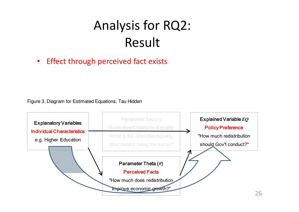
26 Figure 3. Diagram for Estimated Equations, Tau Hidden Explained Variable EQ Policy Preference "How much redistribution should Gov't conduct?" Parameter Theta (θ) Perceived Facts "How much does redistribution improve economic growth?" Parameter Tau (τ) Normative Criteria for Equality "What is the desirable equality, other factors being the same?" Explanatory Variables Individual Characteristics e.g. Higher Education
(S.E.) 0.013 * (0.005) Male Age/100 0.002 (0.048) 0.522 * (0.244) -0.005 (0.048) Married -0.006 (0.017) 0.105 (0.075) -0.007 (0.017) Higher Education 0.031 * (0.013) 0.144 ** (0.054) 0.029 * (0.013) Female Age/100 0.080 (0.054) 0.009 (0.335) 0.080 (0.054) Married -0.008 (0.018) 0.269 ** (0.093) -0.012 (0.018) Higher Education 0.052 ** (0.019) 0.162 * (0.074) 0.050 ** (0.019) Source : JHPS2011-2012 Note: +:p<0.10, *:p<0.05, **:p<0.01 The value of θ is multiplied by 1000 so that the coefficients are decently displayed. θ (Perceived Improvement of Growth by Unit Equalization) --- --- R2 0.011 0.011 For both genders, White Collar and Household Income (Log) are included but turn out to be insignificant. Constant, Male Dummy, and Year Dummy (2012) are also included. 0.016 N of Obs. 3084 3084 3084 Explanatory Variables Model 1 Model 2 Model 3 Dep. Var. Dep. Var. Dep. Var. EQ θ EQ
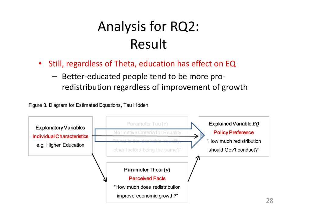
has effect on EQ – Better‐educated people tend to be more pro‐ redistribution regardless of improvement of growth 28 Figure 3. Diagram for Estimated Equations, Tau Hidden Explained Variable EQ Policy Preference "How much redistribution should Gov't conduct?" Parameter Theta (θ) Perceived Facts "How much does redistribution improve economic growth?" Parameter Tau (τ) Normative Criteria for Equality "What is the desirable equality, other factors being the same?" Explanatory Variables Individual Characteristics e.g. Higher Education
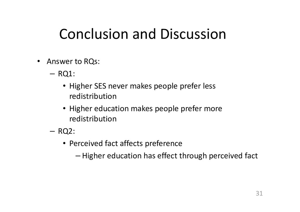
Higher SES never makes people prefer less redistribution • Higher education makes people prefer more redistribution – RQ2: • Perceived fact affects preference – Higher education has effect through perceived fact 31
Redistribution.” Jess Benhabib, Alberto Bisin, and Matthew O. Jackson, eds. Handbook of Social Economics Volume 1A. North Holland: 93‐131. Blekesaune, Morten, and Jill Quadagno. 2003. “Public Attitudes toward Welfare State Policies: A Comparative Analysis of 24 Nations.” European Sociological Review 19 (5): 415‐427. Dallinger, Ursula. 2010. “Public Support for Redistribution: What Explains Cross‐national Differences?” Journal of European Social Policy 20 (4): 333‐349. Giger, Nathalie, and Moira Nelson. 2013. “The Welfare State or the Economy? Preferences, Constituencies, and Strategies for Retrenchment.” European Sociological Review 29 (5): 1083‐1094. Huber, Gregory A., and Celia Paris. 2013. “Assessing the Programmatic Equivalence Assumption in Question Wording Experiments: Understanding Why Americans Like Assistance to the Poor More Than Welfare.” Public Opinion Quarterly 77 (1): 385‐397. Kuziemko, Ilyana, Michael I. Norton, Emmanuel Saez, and Stefanie Stantcheva. 2015. “How Elastic Are Preferences for Redistribution? Evidence from Randomized Survey Experiments.” American Economic Review 105 (4): 1478–1508. Miyauchi, Tamaki. 2013. “Measuring Japanese Constituency Preferences for Income Redistribution Policy and Effects by the Great Earthquake of Eastern Japan in 2011.” Joint Research Center for Panel Studies Discussion Paper Series DP‐2012‐007. Ohtake, Fumio, and Jun Tomioka. 2004. “Who Supports Redistribution?” The Japanese Economic Review 55 (4): 333‐354. Takegawa, Shogo. 2010. “Liberal Preferences and Conservative Policies: The Puzzling Size of Japan’s Welfare State.” Social Science Japan Journal 13 (1): 53‐ 67. Yamamoto, Koji, and Ryotaro Fukahori. 2011. “Methods to Measure and Model Attitude toward Equalization: Searching for Democratically Justifiable Criteria for Policy Evaluation” (in Japanese). Joint Research Center for Panel Studies Discussion Paper Series DP2011‐001. Data Sources Solt, Frederick. 2016. “The Standardized World Income Inequality Database.” Social Science Quarterly 97. SWIID Version 6.0, July 2017. World Bank. 2017. World Development Indicators. (Last Updated September 18, 2017; Datasets are retrieved from https://data.worldbank.org/country/japan).
[email protected] 34 Acknowledgement This study has been supported by JSPS KAKENHI Grant Numbers JP18H00033, JP16H00287, JP11J06528, and JP18830018. The data for this analysis, Japan Household Panel Survey (JHPS/KHPS), was provided by the Keio University Panel Data Research Center. This work was supported by the MEXT‐Supported Program for the Strategic Research Foundation at Private Universities of Japan, 2014‐2018 (S1491003).
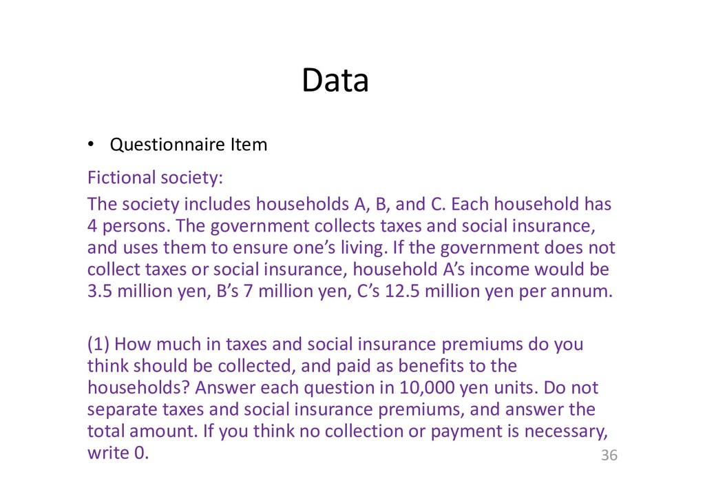
households A, B, and C. Each household has 4 persons. The government collects taxes and social insurance, and uses them to ensure one’s living. If the government does not collect taxes or social insurance, household A’s income would be 3.5 million yen, B’s 7 million yen, C’s 12.5 million yen per annum. (1) How much in taxes and social insurance premiums do you think should be collected, and paid as benefits to the households? Answer each question in 10,000 yen units. Do not separate taxes and social insurance premiums, and answer the total amount. If you think no collection or payment is necessary, write 0.
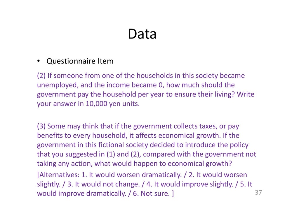
of the households in this society became unemployed, and the income became 0, how much should the government pay the household per year to ensure their living? Write your answer in 10,000 yen units. (3) Some may think that if the government collects taxes, or pay benefits to every household, it affects economical growth. If the government in this fictional society decided to introduce the policy that you suggested in (1) and (2), compared with the government not taking any action, what would happen to economical growth? [Alternatives: 1. It would worsen dramatically. / 2. It would worsen slightly. / 3. It would not change. / 4. It would improve slightly. / 5. It would improve dramatically. / 6. Not sure. ]
model which assumes individual redistributive preference may be affected by the perceived fact about relationship between redistribution and economic growth • Concretely, we assume each person has IEF (Individual Evaluation Function on Status of Society) and one prefers the policy which maximize the evaluated value under perceived restriction 38
evaluated with the equality, EQ, and the economic growth, GR, and also with parameters of normative criteria – There is a perceived restriction in each person’ s mind as follow – The parameter Theta (θ) reflect the perceived fact – Maximizing IEF subject to the restriction, the optimal values of EQ and GR are obtained 39 GR EQ IEF i i i i ) 1 ( ) ( 2 ) ( 0 0 EQ EQ GR GR i i i i i i EQ 2 / ) 1 ( * 0 0 * * ) ( GR EQ EQ GR i i i
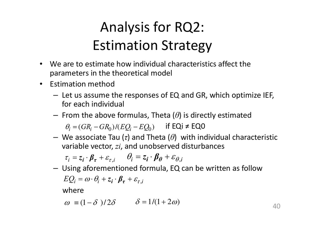
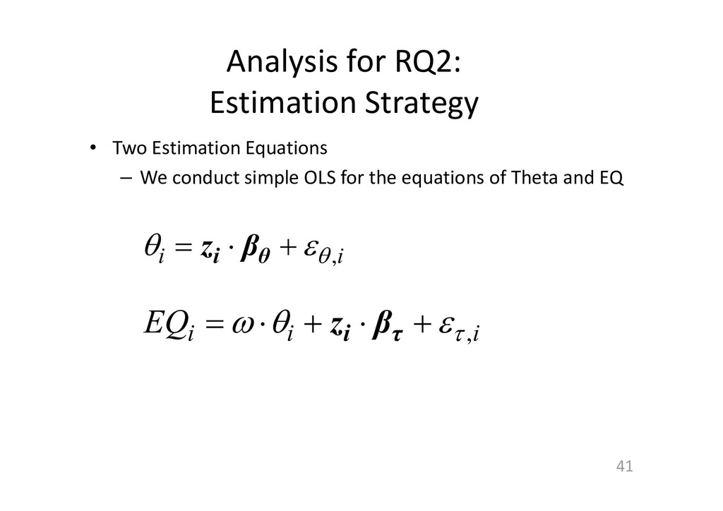
how individual characteristics affect the parameters in the theoretical model • Estimation method – Let us assume the responses of EQ and GR, which optimize IEF, for each individual – From the above formulas, Theta (θ) is directly estimated if EQi ≠ EQ0 – We associate Tau (τ) and Theta (θ) with individual characteristic variable vector, zi, and unobserved disturbances – Using aforementioned formula, EQ can be written as follow where 40 ) /( ) ( 0 0 EQ EQ GR GR i i i i i , τ i β z i i , θ i β z i i i EQ , τ i β z 2 / ) 1 ( ) 2 1 /( 1
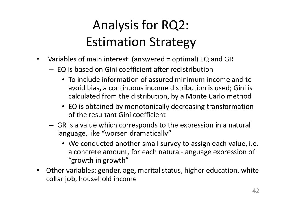
(answered = optimal) EQ and GR – EQ is based on Gini coefficient after redistribution • To include information of assured minimum income and to avoid bias, a continuous income distribution is used; Gini is calculated from the distribution, by a Monte Carlo method • EQ is obtained by monotonically decreasing transformation of the resultant Gini coefficient – GR is a value which corresponds to the expression in a natural language, like “worsen dramatically” • We conducted another small survey to assign each value, i.e. a concrete amount, for each natural‐language expression of “growth in growth” • Other variables: gender, age, marital status, higher education, white collar job, household income 42
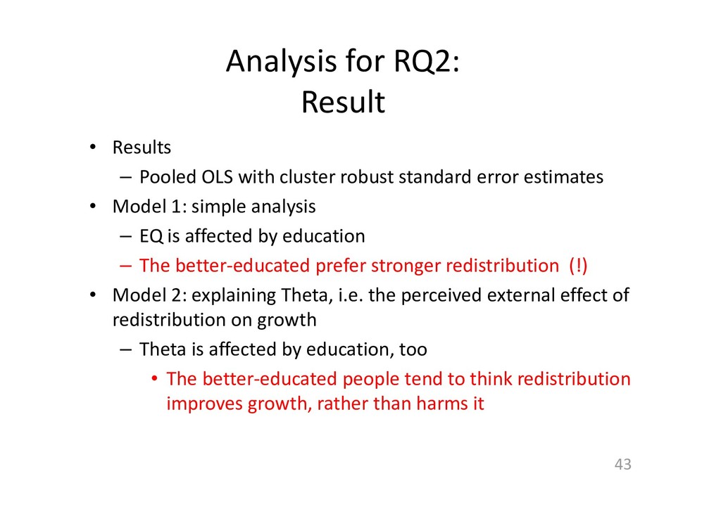
cluster robust standard error estimates • Model 1: simple analysis – EQ is affected by education – The better‐educated prefer stronger redistribution (!) • Model 2: explaining Theta, i.e. the perceived external effect of redistribution on growth – Theta is affected by education, too • The better‐educated people tend to think redistribution improves growth, rather than harms it 43
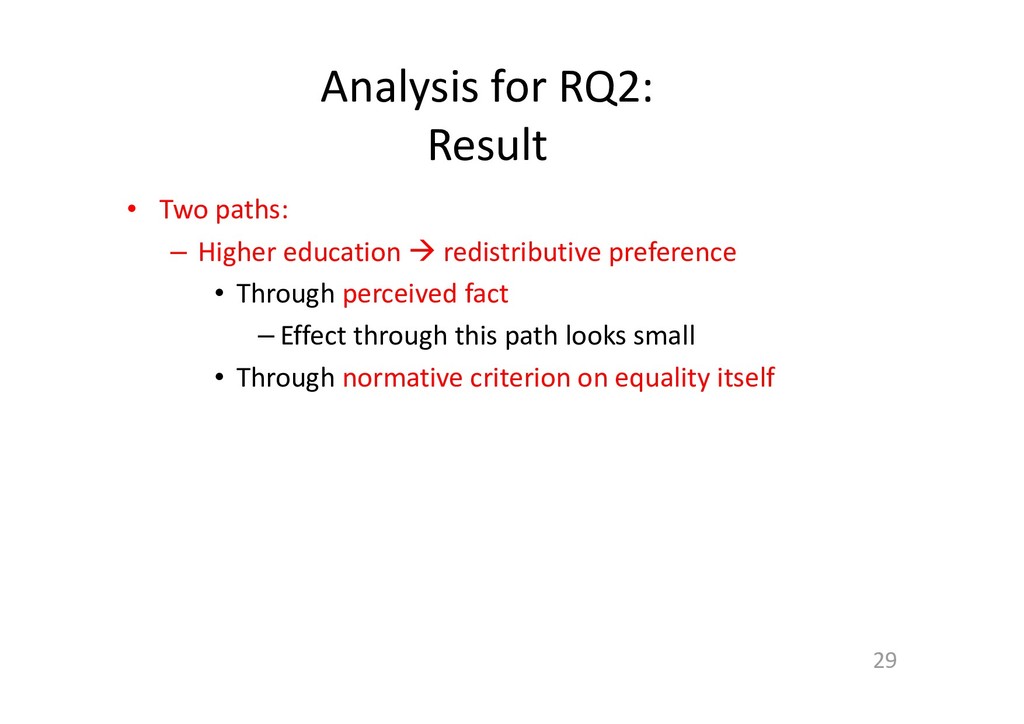
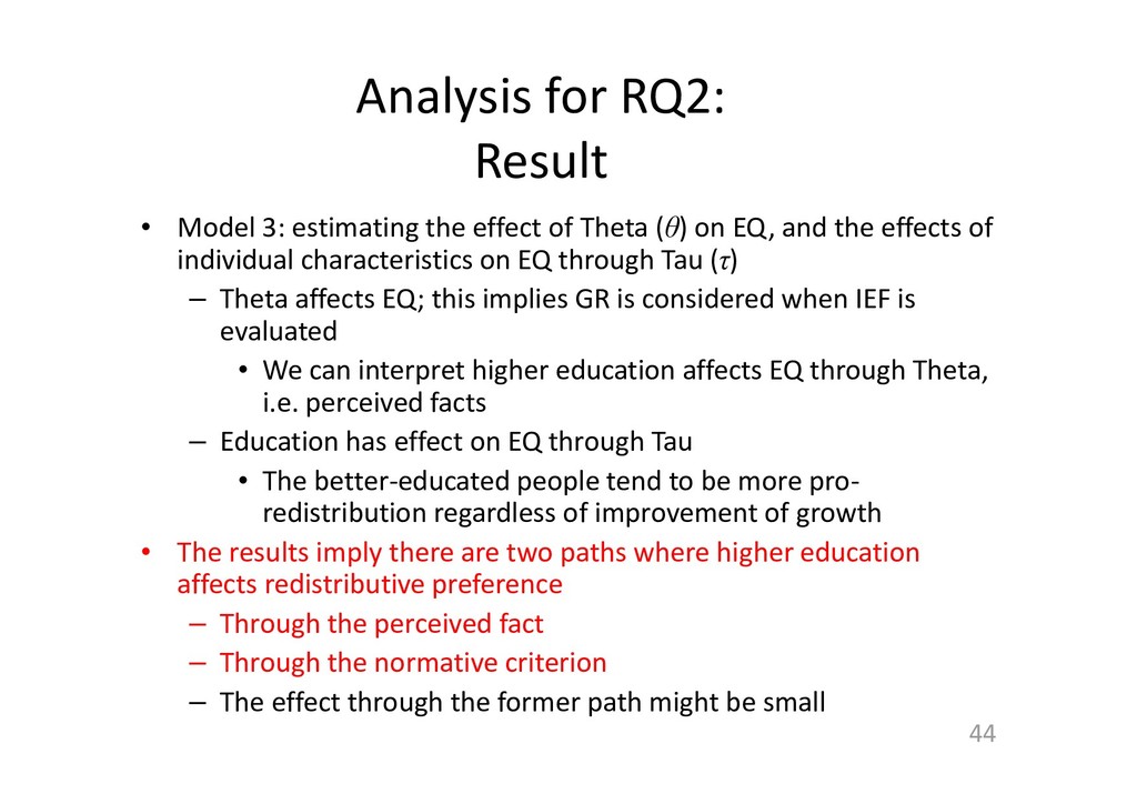
of Theta (θ) on EQ, and the effects of individual characteristics on EQ through Tau (τ) – Theta affects EQ; this implies GR is considered when IEF is evaluated • We can interpret higher education affects EQ through Theta, i.e. perceived facts – Education has effect on EQ through Tau • The better‐educated people tend to be more pro‐ redistribution regardless of improvement of growth • The results imply there are two paths where higher education affects redistributive preference – Through the perceived fact – Through the normative criterion – The effect through the former path might be small 44
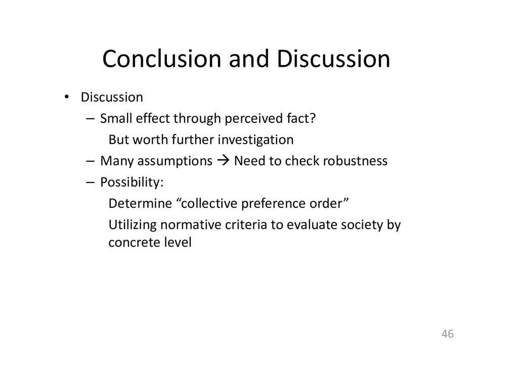
fact? But worth further investigation – Many assumptions Need to check robustness – Possibility: Determine “collective preference order” Utilizing normative criteria to evaluate society by concrete level 46
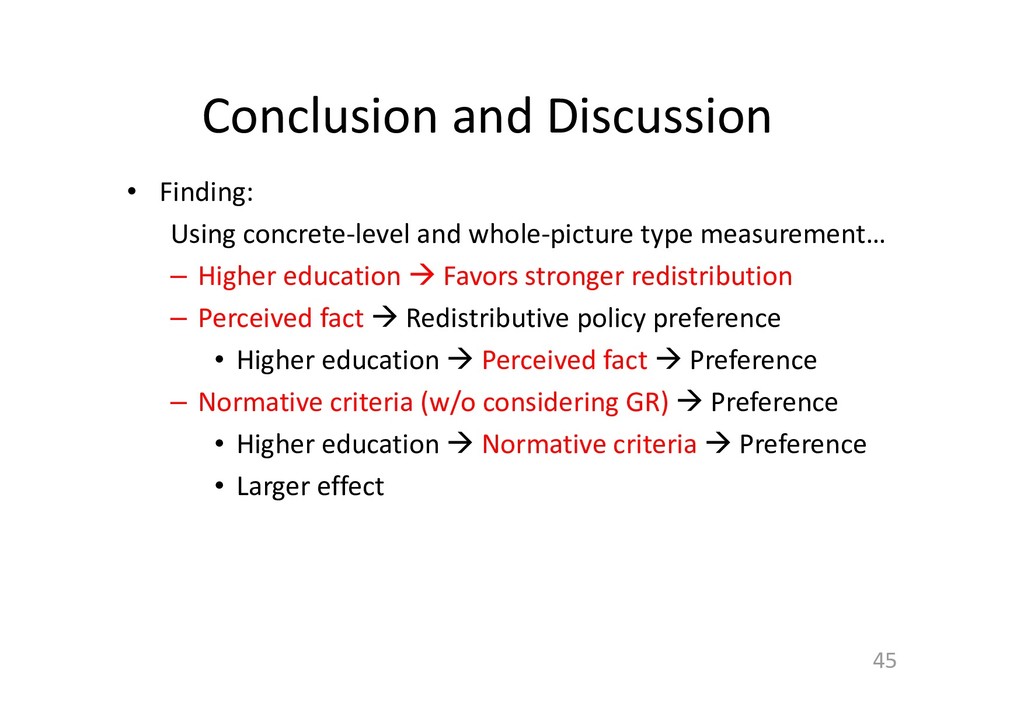
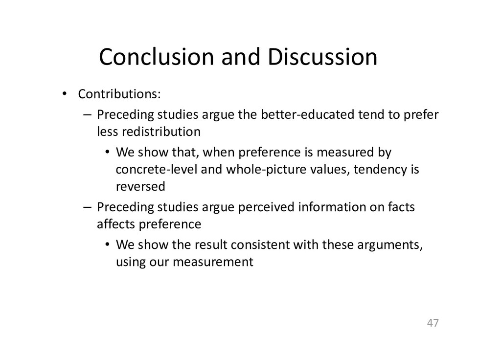
better‐educated tend to prefer less redistribution • We show that, when preference is measured by concrete‐level and whole‐picture values, tendency is reversed – Preceding studies argue perceived information on facts affects preference • We show the result consistent with these arguments, using our measurement 47
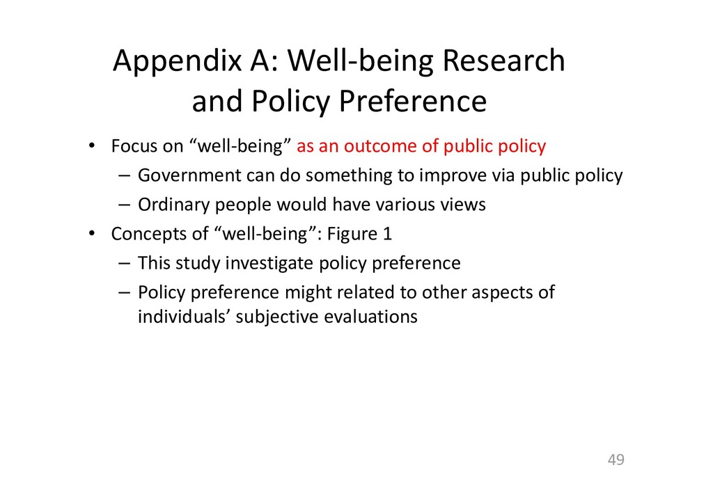
“well‐being” as an outcome of public policy – Government can do something to improve via public policy – Ordinary people would have various views • Concepts of “well‐being”: Figure 1 – This study investigate policy preference – Policy preference might related to other aspects of individuals’ subjective evaluations 49
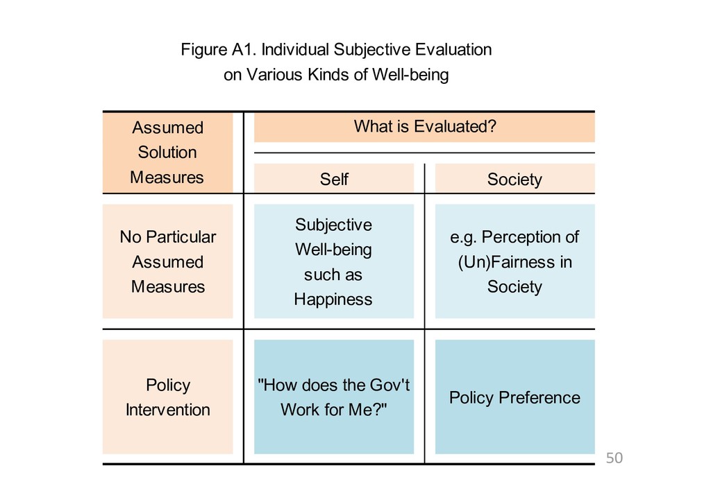
as Happiness e.g. Perception of (Un)Fairness in Society Policy Intervention "How does the Gov't Work for Me?" Policy Preference Assumed Solution Measures What is Evaluated? Figure A1. Individual Subjective Evaluation on Various Kinds of Well-being