Upgrade to Pro — share decks privately, control downloads, hide ads and more …

Concrete and Whole-Picture Type Indices to Measure Policy Preference over Income Redistribution Policy: A Report from Japanese Nationwide Survey Data

Concrete and Whole-Picture Type Indices to Measure Policy Preference over Income Redistribution Policy: A Report from Japanese Nationwide Survey Data

*Presentation at Waseda University, October 29, 2018
This presentation aims to show (1) a set of questionnaire items to measure redistributive policy preference using concrete and whole-picture type indices, which was adopted by a Japanese nationwide survey, (2) the resulted data, and (3) the perspectives for future research of our interest. We emphasize the importance of measuring individuals’ policy preference using concrete-level indices obtained from respondents looking at the whole picture of a society.
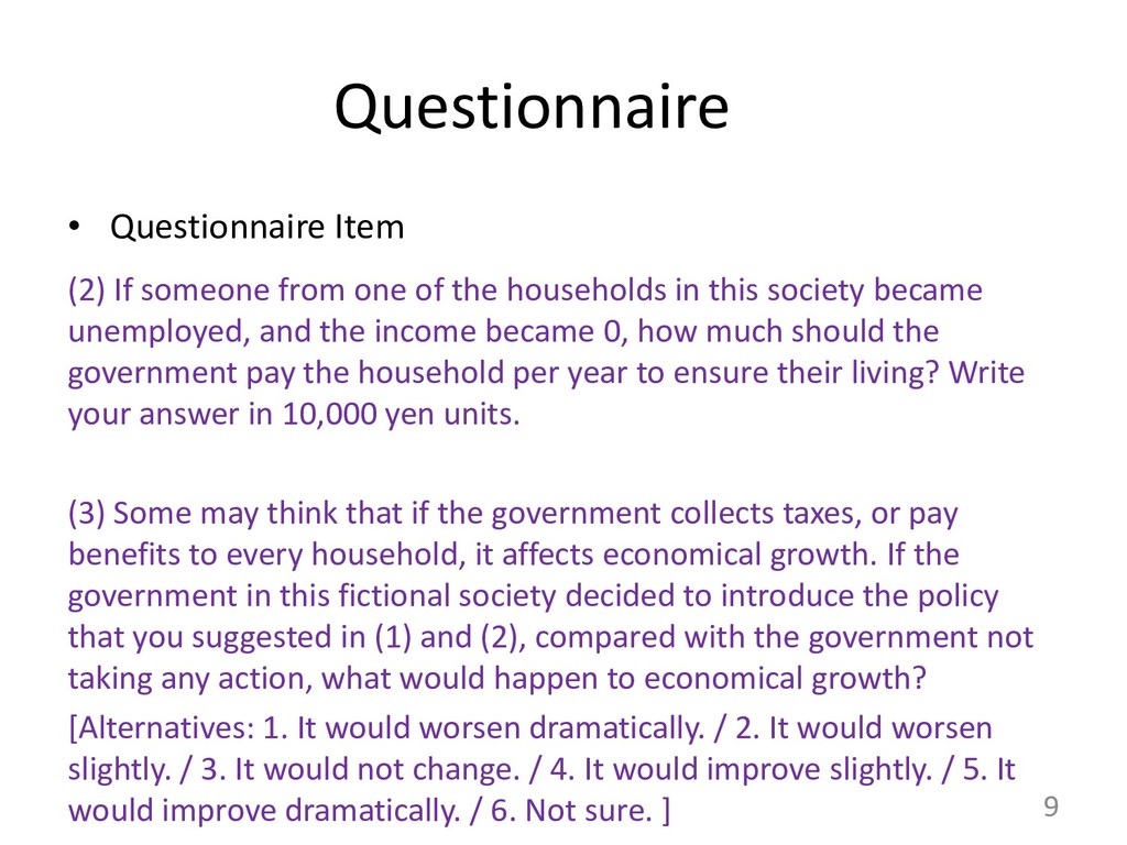
As redistributive preference measures, most studies in literature have utilized “yes/no” responses to some slogan in a natural language. However, when people are to find a political solution in debate on public policy, if it is desirable to make a compromise over concrete levels instead of natural-language slogans, then plausibly we should know how people’s preferences differ in concrete levels of a policy. In other words, we should know how strong/weak redistribution policy people prefer, instead of how strongly/weakly people agree with statements for redistribution.
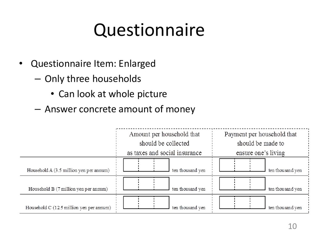
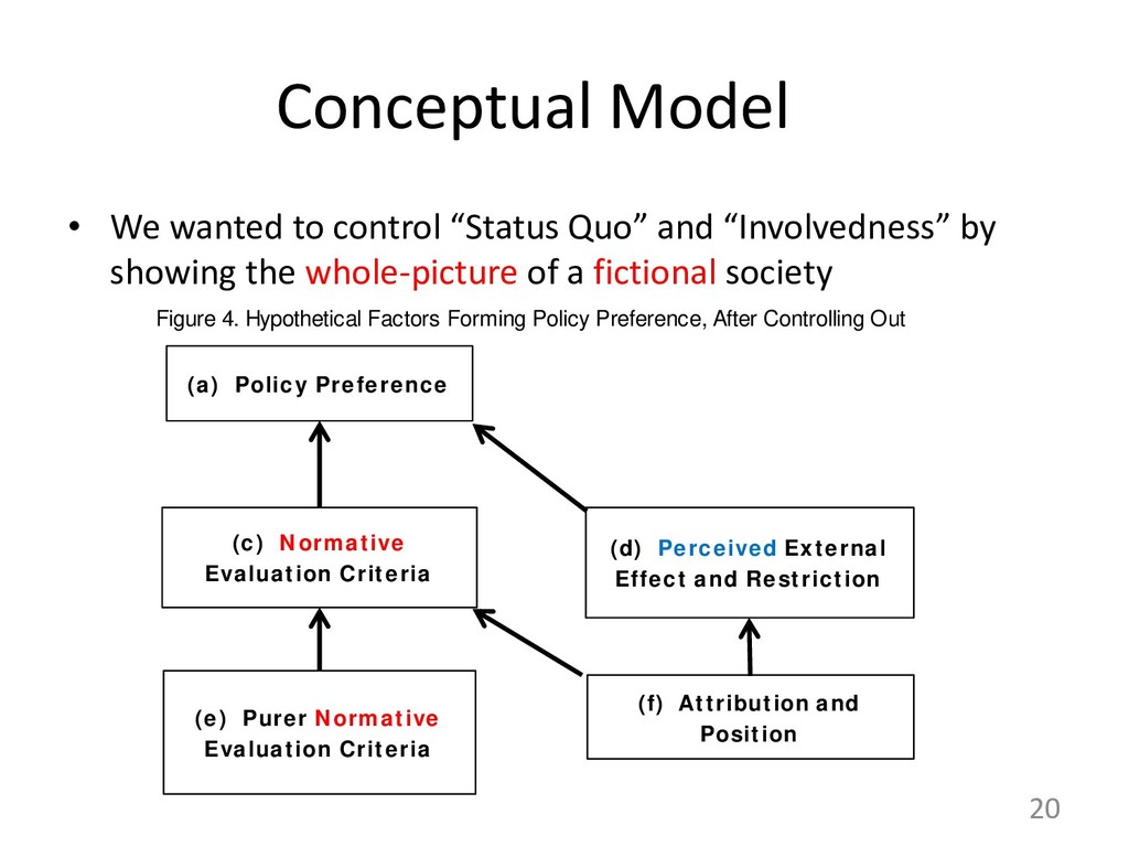
There already exist some studies that deal with such concrete-level indices. Relative to such studies, we aim to contribute by letting respondents answer looking at the whole picture of a society and considering the amount every household should have after redistribution. If it is easier for people to make a compromise about a general status of a society, than about only part of societal status, e.g. about some specific interests, then we should utilize the whole-picture type indices of policy preferences.
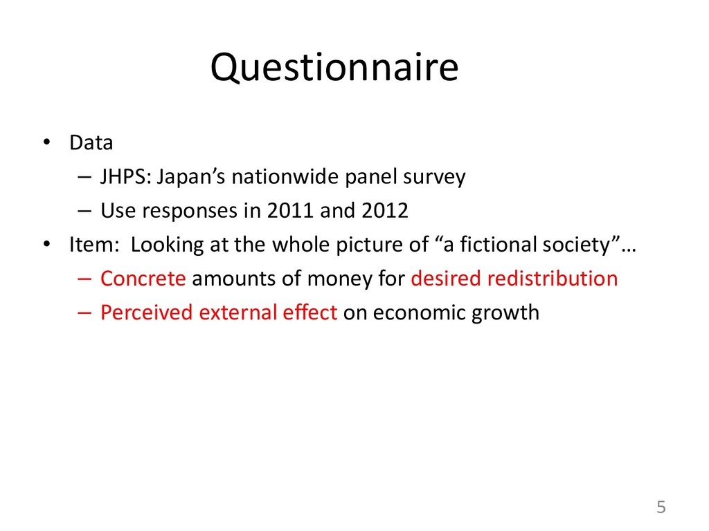
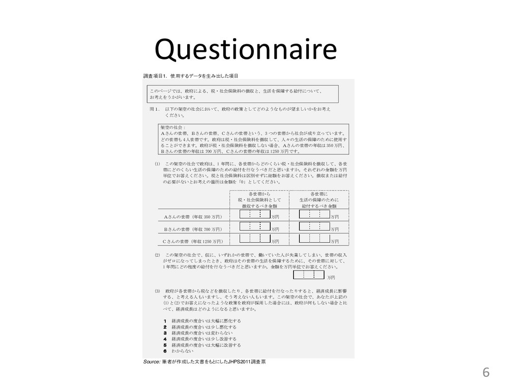
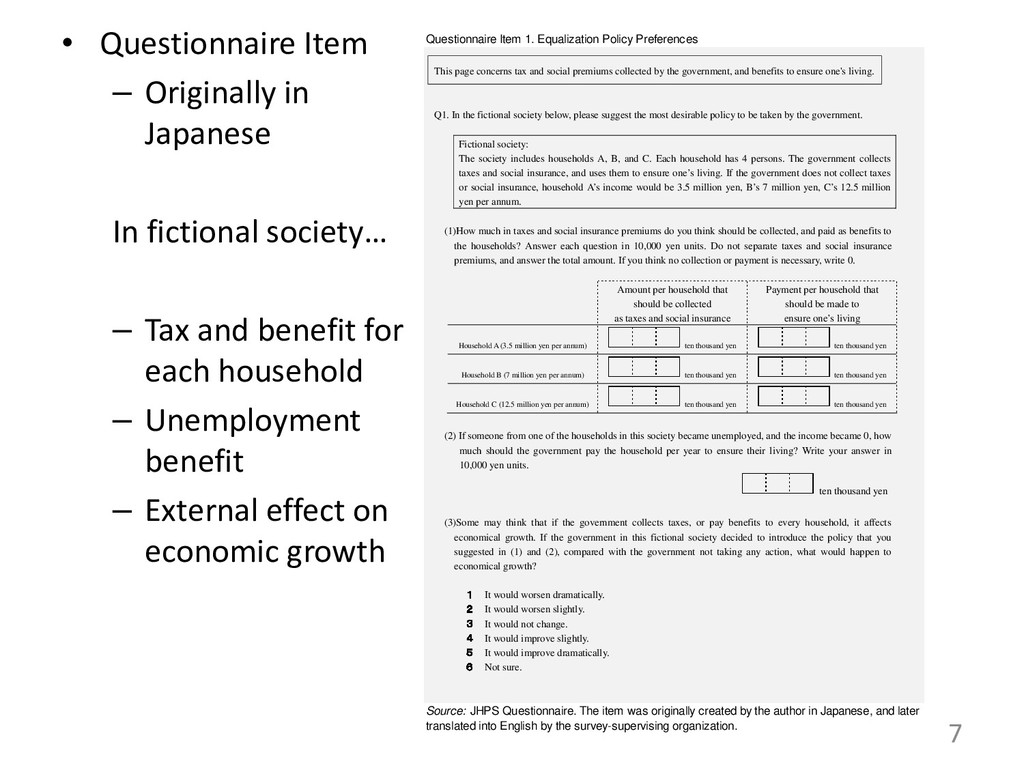
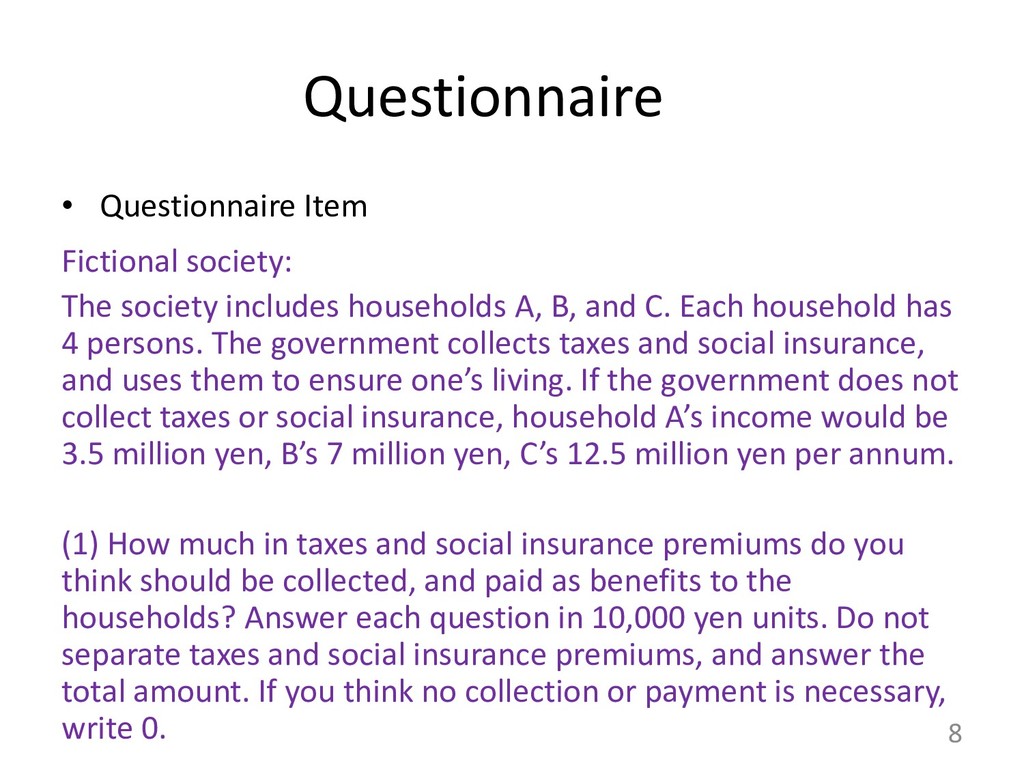
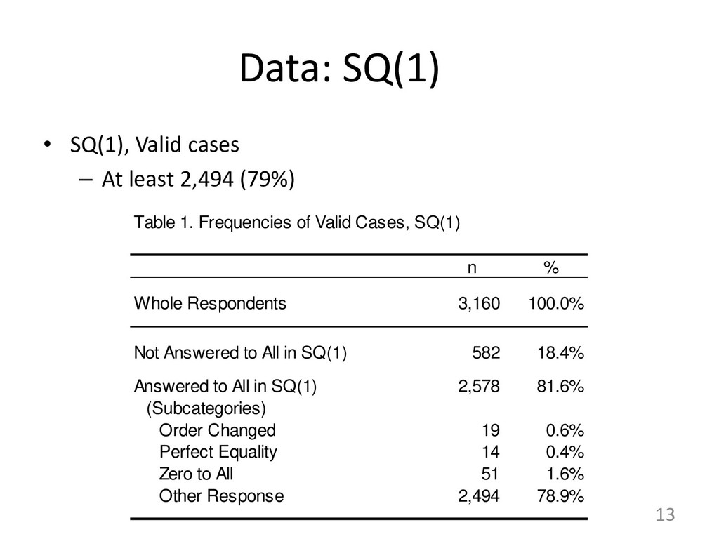
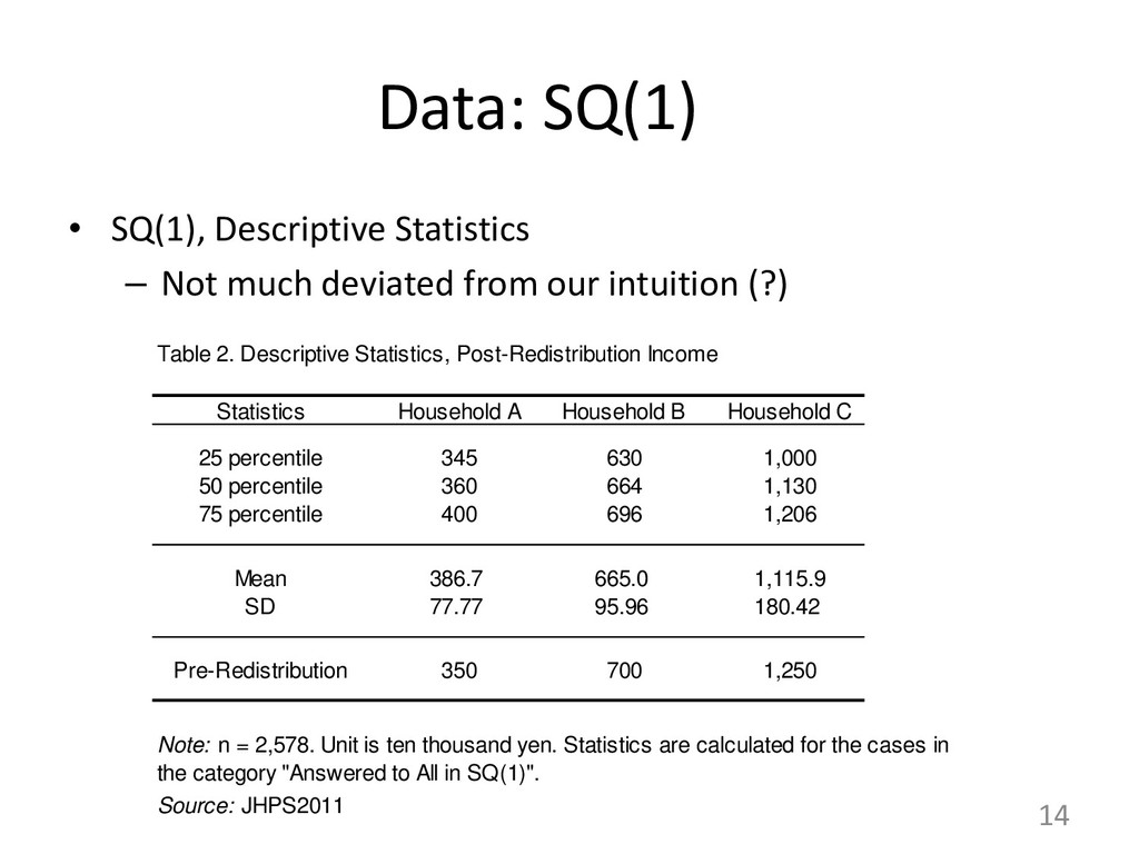
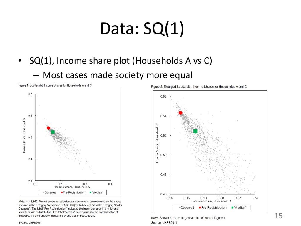
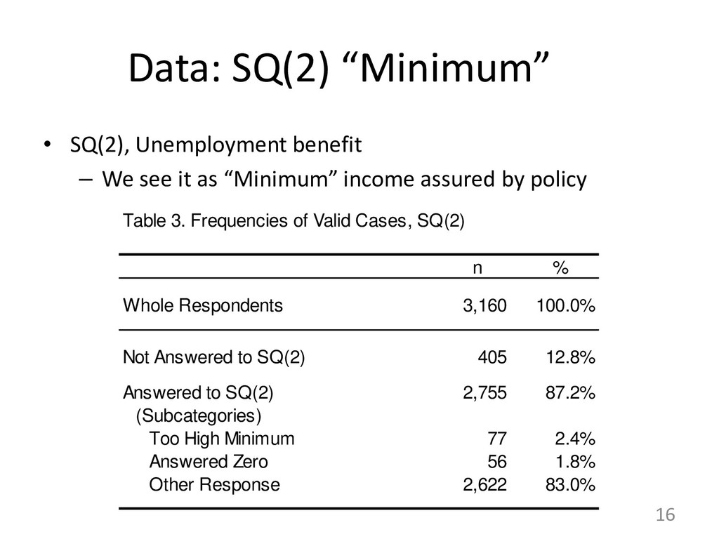
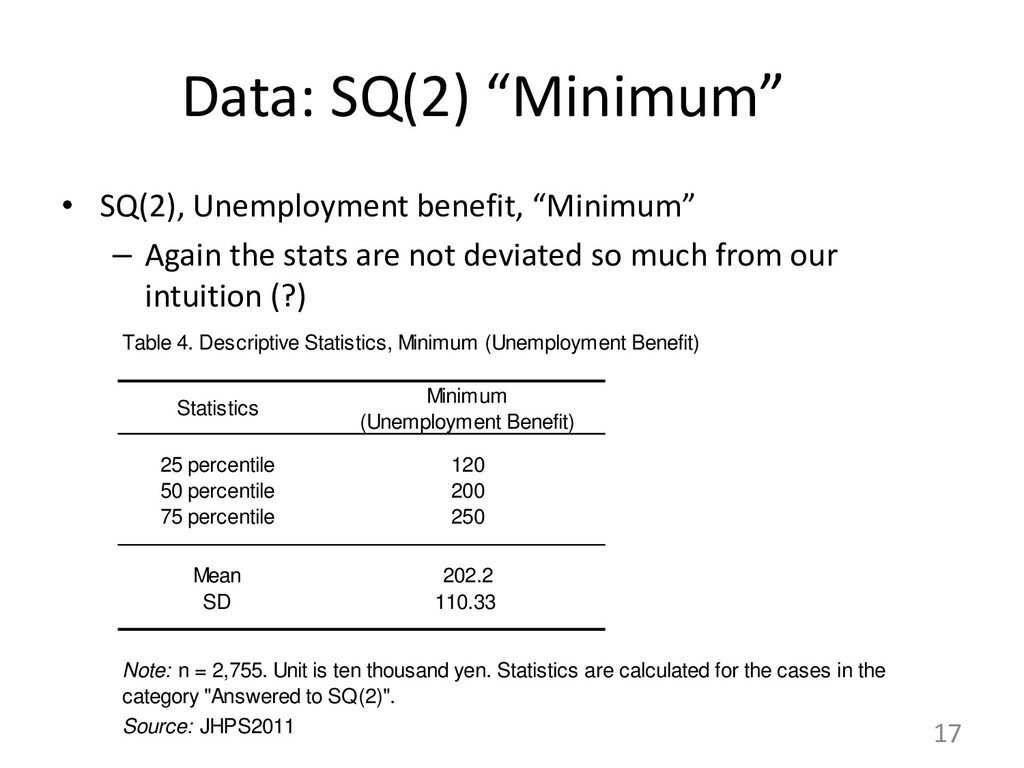
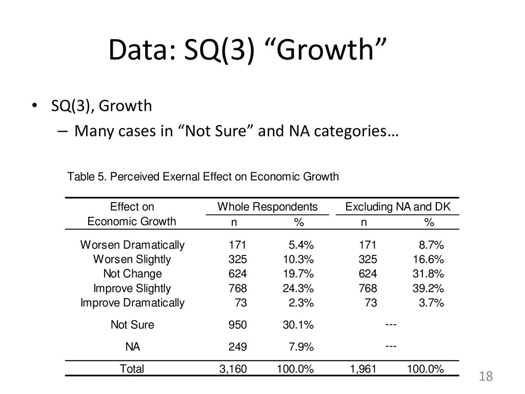
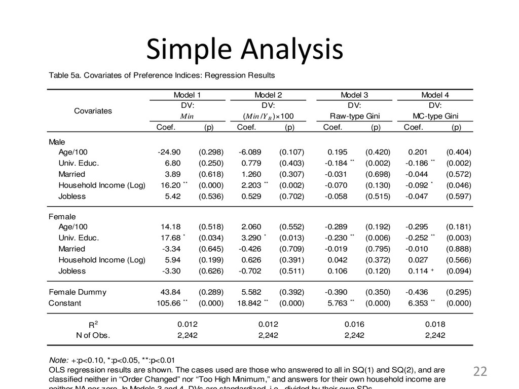
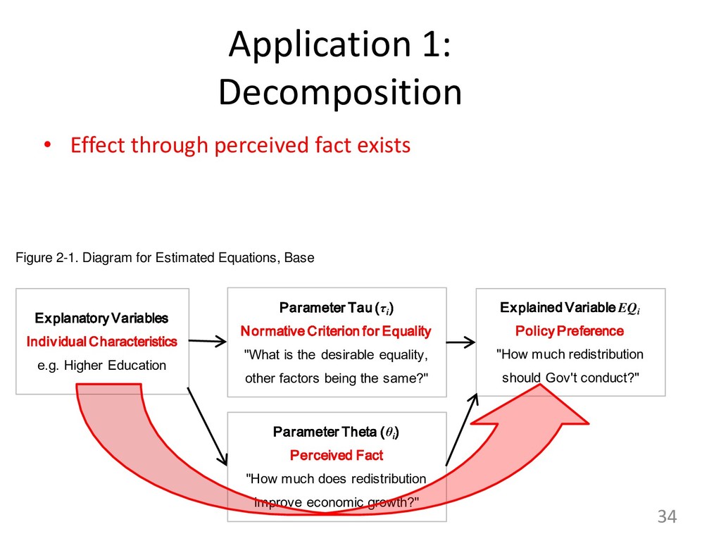
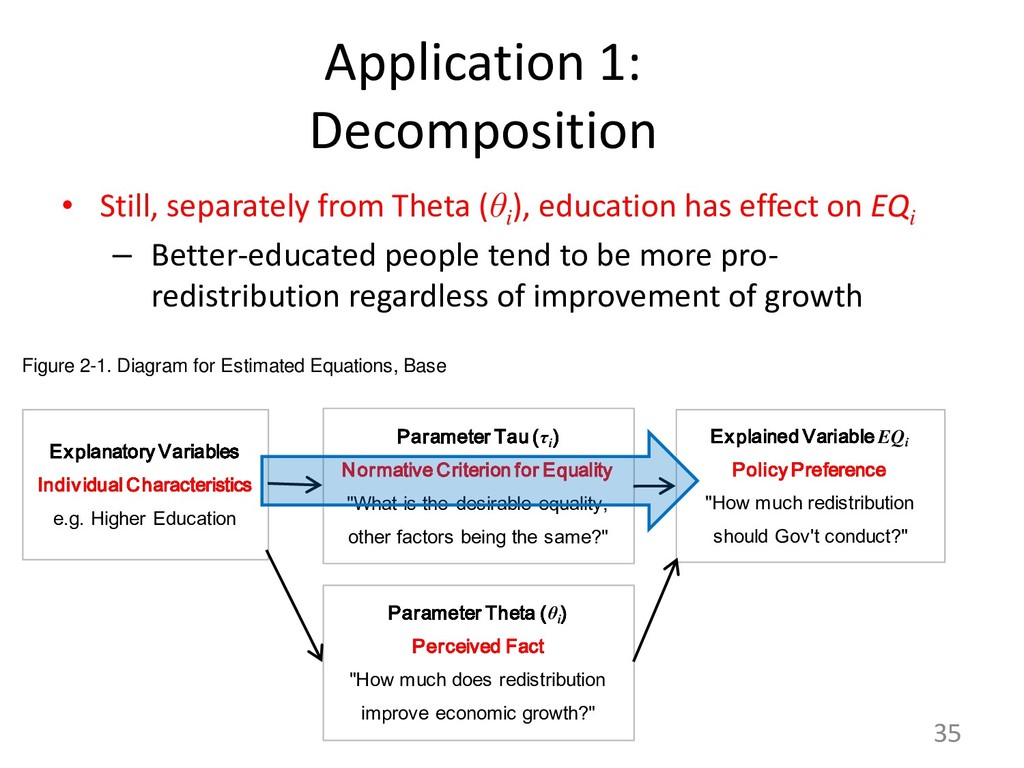
In the presentation, first, we introduce this kind of questionnaire items, where respondents answer the desirable amounts of tax and benefit for each household, and also the unemployment benefit, in a fictional society. The items also measure the perceived external effect of the policy on economic growth. The items were included in JHPS survey conducted in Japan in 2011 and 2012. Second, we show some results as well as descriptive characteristics of the obtained data. Interestingly, we find no evidence that those with lower socio-economic status prefer stronger equalization policy; on the contrary, we find that the better-educated tend to prefer stronger equalization policy.
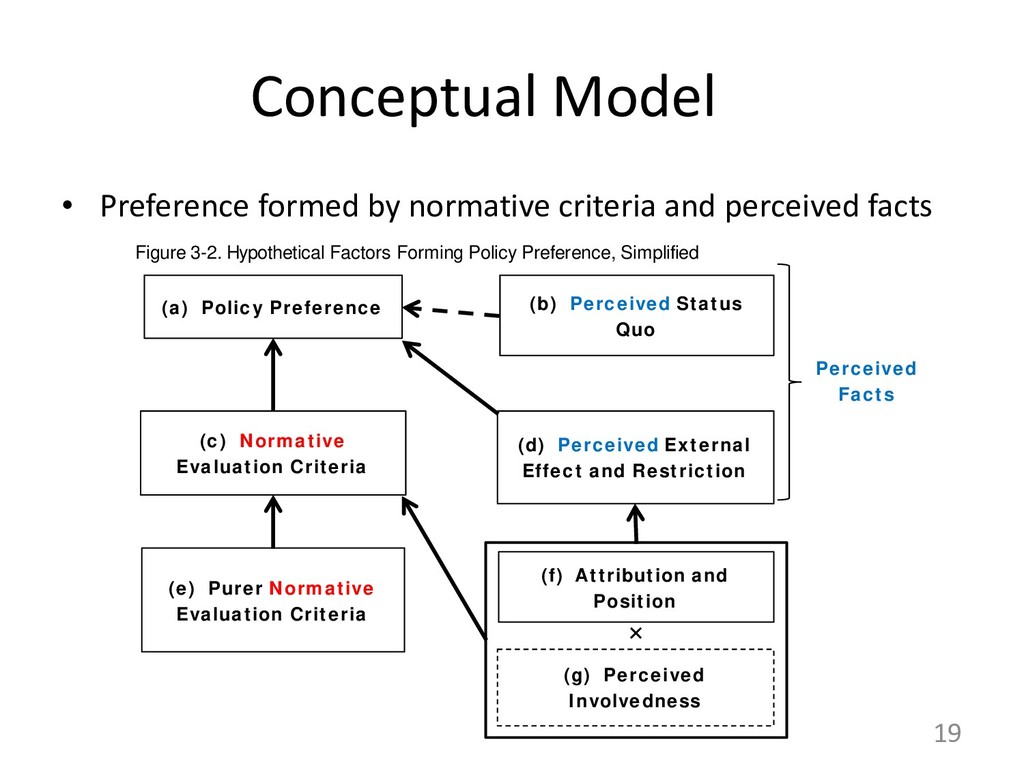
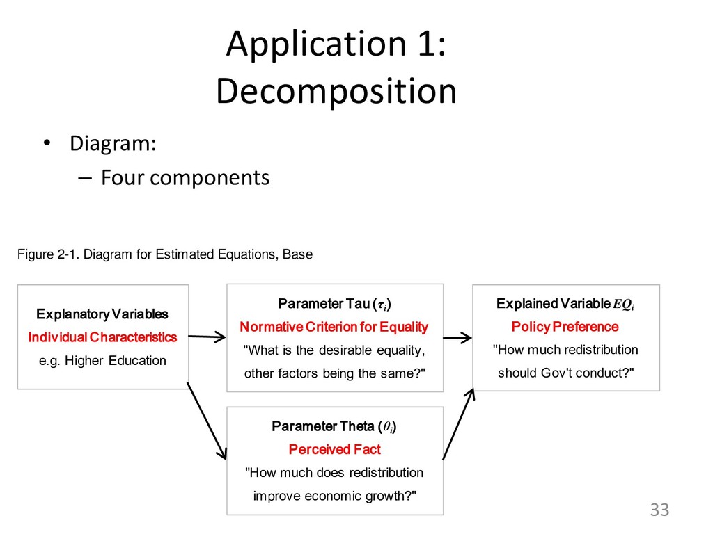
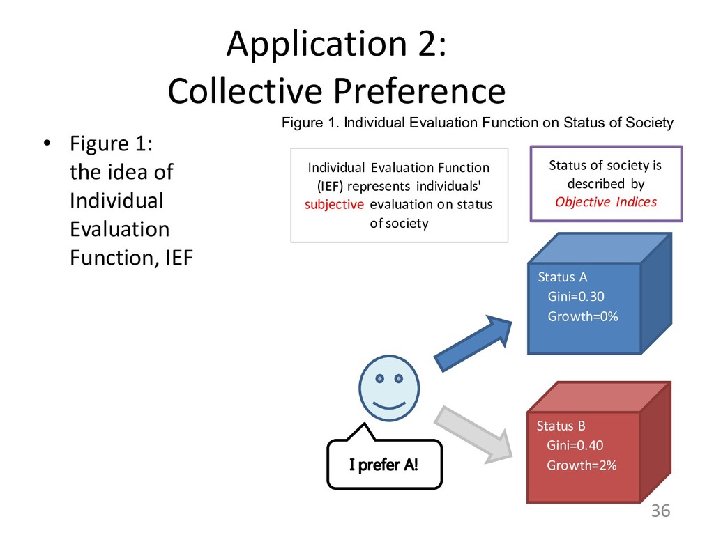
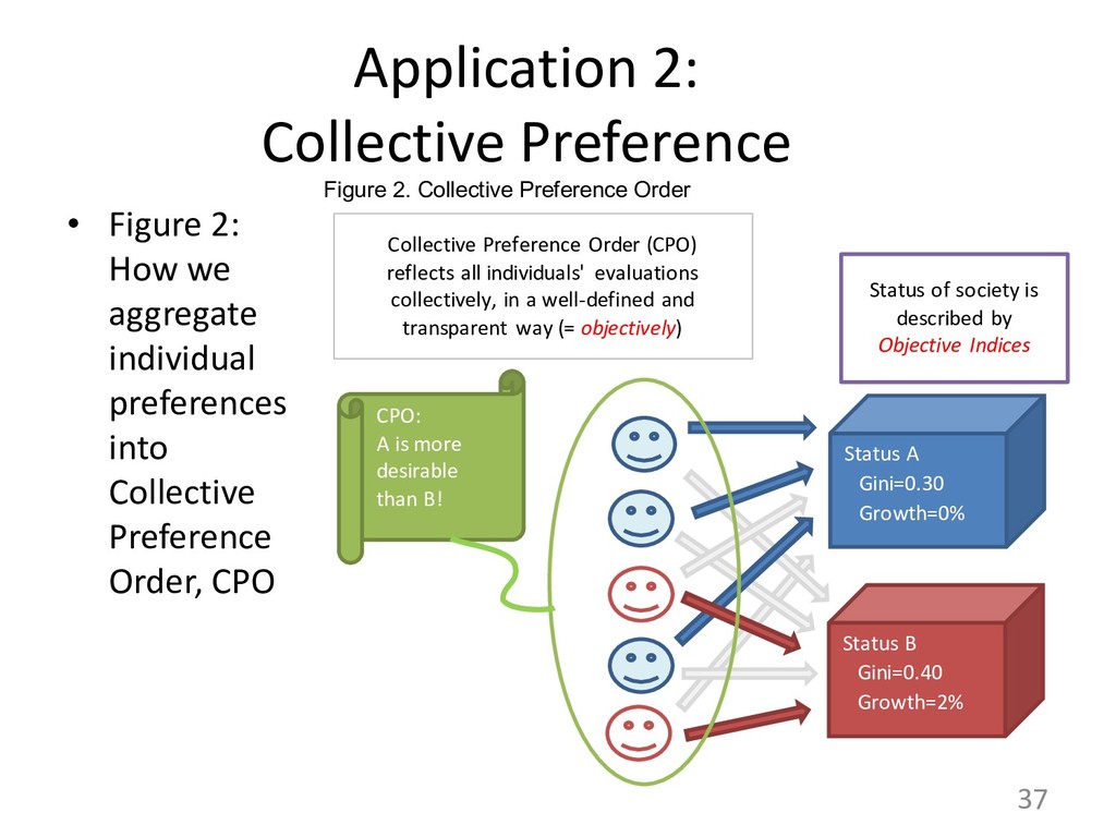
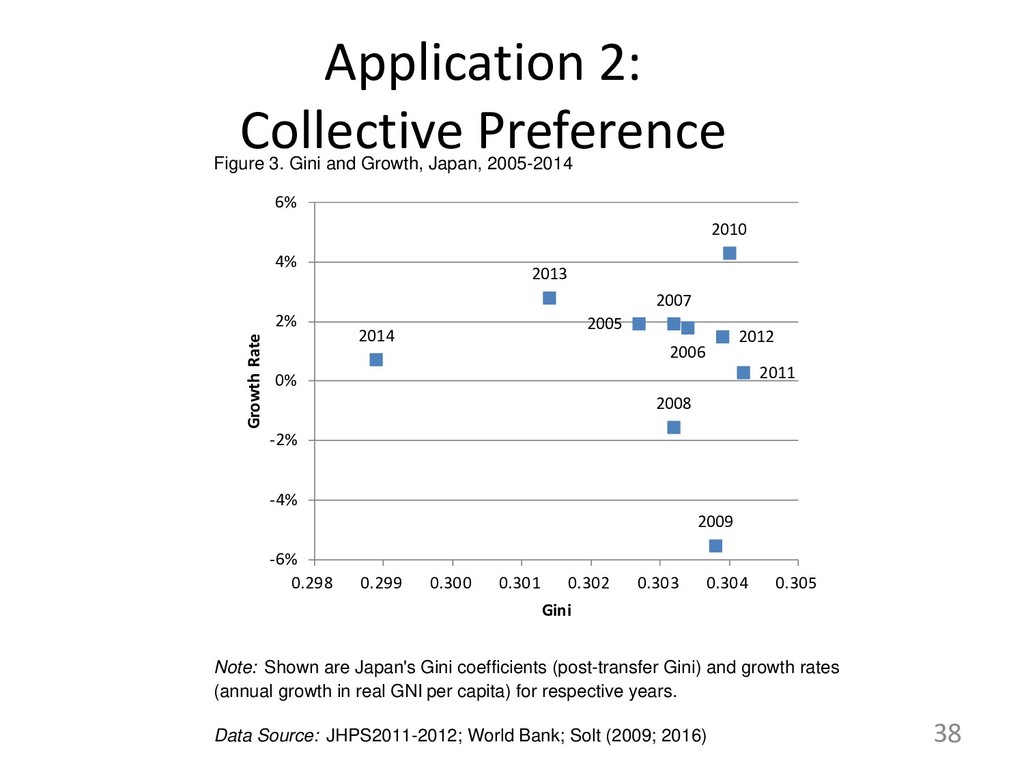
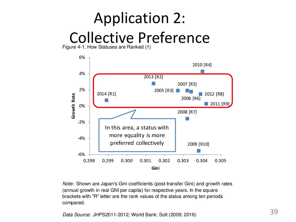
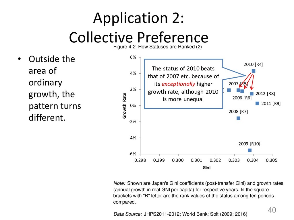
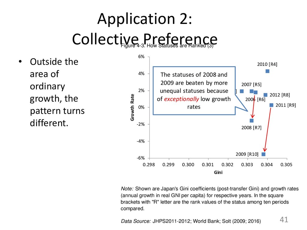
If time allows, we are to show some examples of possible analyses using the data. One of them is to identify the two factors forming the policy preference, namely (a) normative evaluation criteria over societal status and (b) perceived fact on externality of policy. Another is to determine “collective preference order” among various statuses of society, by knowing people’s normative evaluation on various sets of concrete indices about a whole society, and then aggregating such evaluations collectively.
Our presentation is open to discussion, not necessarily coming with a well-defined framing as an academic paper.

Koji Yamamoto

October 29, 2018
Tweet

More Decks by Koji Yamamoto

Other Decks in Research

Transcript

  1. Concrete and Whole-Picture Type Indices to Measure Policy Preference over

    Income Redistribution Policy: A Report from Japanese Nationwide Survey Data Koji YAMAMOTO (Hylab LLP and Senshu University) Presentation at Waseda University, October 29, 2018
  2. Introduction • Focus: – Preference for redistribution policy • Background:

    – How could people come close to agreement, instead of conflict, over public policy? 2
  3. Introduction • What do we need? – Measurement: • Concrete

    level “How strong redistribution one prefers” Not “How strongly one agrees with redistribution” • Respondents look at “whole picture” of society “Be-the-Government” 3
  4. Introduction • Concrete level – Usually policy implementations involves “levels”

    – Natural language expressions are subject to different interpretations • Whole-picture – Some may think “if richer people pay much tax, then poorer people should be left as they are, but if we can make the rich pay more tax, then the poor should receive more” – You can do that by the whole-picture answers 4
  5. Questionnaire • Data – JHPS: Japan’s nationwide panel survey –

    Use responses in 2011 and 2012 • Item: Looking at the whole picture of “a fictional society”… – Concrete amounts of money for desired redistribution – Perceived external effect on economic growth 5
  6. Questionnaire 6 調査項目1. 使用するデータを生み出した項目 Source: 筆者が作成した文書をもとにしたJHPS2011調査票 このページでは、政府による、税・社会保険料の徴収と、生活を保障する給付について、 お考えをうかがいます。 問1. 以下の架空の社会において、政府の政策としてどのようなものが望ましいかをお考え ください。

    架空の社会: Aさんの世帯、Bさんの世帯、Cさんの世帯という、3 つの世帯から社会が成り立っています。 どの世帯も 4 人世帯です。政府は税・社会保険料を徴収して、人々の生活の保障のために使用す ることができます。政府が税・社会保険料を徴収しない場合、Aさんの世帯の年収は 350 万円、 Bさんの世帯の年収は 700 万円、Cさんの世帯の年収は 1250 万円です。 (1) この架空の社会で政府は、1 年間に、各世帯からどのくらい税・社会保険料を徴収して、各世 帯にどのくらい生活の保障のための給付を行なうべきだと思いますか。それぞれの金額を万円 単位でお答えください。税と社会保険料は区別せずに総額をお答えください。徴収または給付 の必要がないとお考えの箇所は金額を「0」としてください。 各世帯から 税・社会保険料として 徴収するべき金額 各世帯に 生活の保障のために 給付するべき金額 Aさんの世帯(年収 350 万円) 万円 万円 Bさんの世帯(年収 700 万円) 万円 万円 Cさんの世帯(年収 1250 万円) 万円 万円 (2) この架空の社会で、仮に、いずれかの世帯で、働いていた人が失業してしまい、世帯の収入 がゼロになってしまったとき、政府はその世帯の生活を保障するために、その世帯に対して、 1 年間にどの程度の給付を行なうべきだと思いますか。金額を万円単位でお答えください。 万円 (3) 政府が各世帯から税などを徴収したり、各世帯に給付を行なったりすると、経済成長に影響 する、と考える人もいますし、そう考えない人もいます。この架空の社会で、あなたが上記の (1)と(2)でお答えになったような政策を政府が採用した場合には、政府が何もしない場合と比 べて、経済成長はどのようになると思いますか。 1 経済成長の度合いは大幅に悪化する 2 経済成長の度合いは少し悪化する 3 経済成長の度合いは変わらない 4 経済成長の度合いは少し改善する 5 経済成長の度合いは大幅に改善する 6 わからない
  7. • Questionnaire Item – Originally in Japanese In fictional society…

    – Tax and benefit for each household – Unemployment benefit – External effect on economic growth 7 Questionnaire Item 1. Equalization Policy Preferences Source: JHPS Questionnaire. The item was originally created by the author in Japanese, and later translated into English by the survey-supervising organization. This page concerns tax and social premiums collected by the government, and benefits to ensure one's living. Q1. In the fictional society below, please suggest the most desirable policy to be taken by the government. Fictional society: The society includes households A, B, and C. Each household has 4 persons. The government collects taxes and social insurance, and uses them to ensure one’s living. If the government does not collect taxes or social insurance, household A’s income would be 3.5 million yen, B’s 7 million yen, C’s 12.5 million yen per annum. (1)How much in taxes and social insurance premiums do you think should be collected, and paid as benefits to the households? Answer each question in 10,000 yen units. Do not separate taxes and social insurance premiums, and answer the total amount. If you think no collection or payment is necessary, write 0. Amount per household that should be collected as taxes and social insurance Payment per household that should be made to ensure one’s living Household A (3.5 million yen per annum) ten thousand yen ten thousand yen Household B (7 million yen per annum) ten thousand yen ten thousand yen Household C (12.5 million yen per annum) ten thousand yen ten thousand yen (2) If someone from one of the households in this society became unemployed, and the income became 0, how much should the government pay the household per year to ensure their living? Write your answer in 10,000 yen units. ten thousand yen (3)Some may think that if the government collects taxes, or pay benefits to every household, it affects economical growth. If the government in this fictional society decided to introduce the policy that you suggested in (1) and (2), compared with the government not taking any action, what would happen to economical growth? 1 It would worsen dramatically. 2 It would worsen slightly. 3 It would not change. 4 It would improve slightly. 5 It would improve dramatically. 6 Not sure.
  8. Questionnaire • Questionnaire Item 8 Fictional society: The society includes

    households A, B, and C. Each household has 4 persons. The government collects taxes and social insurance, and uses them to ensure one’s living. If the government does not collect taxes or social insurance, household A’s income would be 3.5 million yen, B’s 7 million yen, C’s 12.5 million yen per annum. (1) How much in taxes and social insurance premiums do you think should be collected, and paid as benefits to the households? Answer each question in 10,000 yen units. Do not separate taxes and social insurance premiums, and answer the total amount. If you think no collection or payment is necessary, write 0.
  9. Questionnaire • Questionnaire Item 9 (2) If someone from one

    of the households in this society became unemployed, and the income became 0, how much should the government pay the household per year to ensure their living? Write your answer in 10,000 yen units. (3) Some may think that if the government collects taxes, or pay benefits to every household, it affects economical growth. If the government in this fictional society decided to introduce the policy that you suggested in (1) and (2), compared with the government not taking any action, what would happen to economical growth? [Alternatives: 1. It would worsen dramatically. / 2. It would worsen slightly. / 3. It would not change. / 4. It would improve slightly. / 5. It would improve dramatically. / 6. Not sure. ]
  10. Questionnaire • Questionnaire Item: Enlarged – Only three households •

    Can look at whole picture – Answer concrete amount of money 10
  11. Questionnaire • Too simple? – OK, and what about natural-language

    quenstions? • Too complicated? – I know, and how can we know what we want to know? • Experiment? Conjoint? 11
  12. Questionnaire • What we will measure: Policy implementation – Not

    “choosing desirable income distribution” – Not “personal satisfaction with income” • Someone may think… – “Personally, low income would be fine, but the government should redistribute more” – “Personally, I would need more money, but the that’s not the government should do” • We will see policy implementation 12
  13. Data: SQ(1) • SQ(1), Valid cases – At least 2,494

    (79%) 13 Table 1. Frequencies of Valid Cases, SQ(1) n % Whole Respondents 3,160 100.0% Not Answered to All in SQ(1) 582 18.4% Answered to All in SQ(1) 2,578 81.6% (Subcategories) Order Changed 19 0.6% Perfect Equality 14 0.4% Zero to All 51 1.6% Other Response 2,494 78.9%
  14. Data: SQ(1) • SQ(1), Descriptive Statistics – Not much deviated

    from our intuition (?) 14 Table 2. Descriptive Statistics, Post-Redistribution Income Statistics Household A Household B Household C 25 percentile 345 630 1,000 50 percentile 360 664 1,130 75 percentile 400 696 1,206 Mean 386.7 665.0 1,115.9 SD 77.77 95.96 180.42 Pre-Redistribution 350 700 1,250 Source: JHPS2011 Note: n = 2,578. Unit is ten thousand yen. Statistics are calculated for the cases in the category "Answered to All in SQ(1)".
  15. Data: SQ(1) • SQ(1), Income share plot (Households A vs

    C) – Most cases made society more equal 15
  16. Data: SQ(2) “Minimum” • SQ(2), Unemployment benefit – We see

    it as “Minimum” income assured by policy 16 Table 3. Frequencies of Valid Cases, SQ(2) n % Whole Respondents 3,160 100.0% Not Answered to SQ(2) 405 12.8% Answered to SQ(2) 2,755 87.2% (Subcategories) Too High Minimum 77 2.4% Answered Zero 56 1.8% Other Response 2,622 83.0%
  17. Data: SQ(2) “Minimum” • SQ(2), Unemployment benefit, “Minimum” – Again

    the stats are not deviated so much from our intuition (?) 17 Table 4. Descriptive Statistics, Minimum (Unemployment Benefit) Statistics Minimum (Unemployment Benefit) 25 percentile 120 50 percentile 200 75 percentile 250 Mean 202.2 SD 110.33 Source: JHPS2011 Note: n = 2,755. Unit is ten thousand yen. Statistics are calculated for the cases in the category "Answered to SQ(2)".
  18. Data: SQ(3) “Growth” • SQ(3), Growth – Many cases in

    “Not Sure” and NA categories… 18 Table 5. Perceived Exernal Effect on Economic Growth Worsen Dramatically 171 5.4% 171 8.7% Worsen Slightly 325 10.3% 325 16.6% Not Change 624 19.7% 624 31.8% Improve Slightly 768 24.3% 768 39.2% Improve Dramatically 73 2.3% 73 3.7% Not Sure 950 30.1% NA 249 7.9% Total 3,160 100.0% 1,961 100.0% --- --- Effect on Economic Growth Excluding NA and DK Whole Respondents n % n %
  19. Conceptual Model • Preference formed by normative criteria and perceived

    facts 19 Figure 3-2. Hypothetical Factors Forming Policy Preference, Simplified (a) Policy Preference (d) Perceived External Effect and Restriction (c) Normative Evaluation Criteria (e) Purer Normative Evaluation Criteria (f) Attribution and Position (b) Perceived Status Quo Perceived Facts (g) Perceived Involvedness ×
  20. Conceptual Model • We wanted to control “Status Quo” and

    “Involvedness” by showing the whole-picture of a fictional society 20 Figure 4. Hypothetical Factors Forming Policy Preference, After Controlling Out (a) Policy Preference (d) Perceived External Effect and Restriction (c) Normative Evaluation Criteria (e) Purer Normative Evaluation Criteria (f) Attribution and Position
  21. Simple Analysis • OLS • DV: – Minimum – Minimum

    / (Household B’ income after redist.) – Raw-type Gini: Gini coefficient calculated from the three household income values after redist. • Covariates: – Age, Univ. Educ., Married dummy, Household Inocme (Logged), Jobless dummy, Female dummy – Separate parameters between both genders 21
  22. Simple Analysis 22 Table 5a. Covariates of Preference Indices: Regression

    Results Coef. (p) Coef. (p) Coef. (p) Coef. (p) Male Age/100 -24.90 (0.298) -6.089 (0.107) 0.195 (0.420) 0.201 (0.404) Univ. Educ. 6.80 (0.250) 0.779 (0.403) -0.184 ** (0.002) -0.186 ** (0.002) Married 3.89 (0.618) 1.260 (0.307) -0.031 (0.698) -0.044 (0.572) Household Income (Log) 16.20 ** (0.000) 2.203 ** (0.002) -0.070 (0.130) -0.092 * (0.046) Jobless 5.42 (0.536) 0.529 (0.702) -0.058 (0.515) -0.047 (0.597) Female Age/100 14.18 (0.518) 2.060 (0.552) -0.289 (0.192) -0.295 (0.181) Univ. Educ. 17.68 * (0.034) 3.290 * (0.013) -0.230 ** (0.006) -0.252 ** (0.003) Married -3.34 (0.645) -0.426 (0.709) -0.019 (0.795) -0.010 (0.888) Household Income (Log) 5.94 (0.199) 0.626 (0.391) 0.042 (0.372) 0.027 (0.566) Jobless -3.30 (0.626) -0.702 (0.511) 0.106 (0.120) 0.114 + (0.094) Female Dummy 43.84 (0.289) 5.582 (0.392) -0.390 (0.350) -0.436 (0.295) Constant 105.66 ** (0.000) 18.842 ** (0.000) 5.763 ** (0.000) 6.353 ** (0.000) 2,242 Note: +:p<0.10, *:p<0.05, **:p<0.01 OLS regression results are shown. The cases used are those who answered to all in SQ(1) and SQ(2), and are classified neither in “Order Changed” nor “Too High Minimum,” and answers for their own household income are Model 3 Model 4 DV: DV: Raw-type Gini MC-type Gini 0.016 0.018 2,242 R2 0.012 0.012 N of Obs. 2,242 2,242 Covariates Model 1 Model 2 DV: DV: Min (Min /YB )×100
  23. Simple Analysis • No evidence that “those with lower SES

    prefer stronger redistribution” • Male: – Higher Household income  Higher Minimum • Female: – Univ. Educ.  Higher Minimum • Both genders: – Univ. Educ.  Lower post-redist. Gini • Yes, R-squared is small… – There is no clear systematic difference in concrete-amount preference? 23
  24. Considering “Minimum” • How to integrate minimum into other 3

    household income values? – Respondents answered the packaged of the policy • Assume continuous income distribution – Continuous dist.: • More comparable with real societies (Small freq. makes Gini biased) • Introduce the idea of Income Transformation Function (ITF) 24
  25. Considering “Minimum” • Introduce the idea of Income Transformation Function

    (ITF) 25 Figure 1. Income Transformation Function (ITF), Setting Various Minimum Income Values 0 250 500 750 1,000 1,250 0 250 500 750 1,000 1,250 Post-Redistribution Income Pre-Redistribution Income (Unit: Ten Thousand Yen) Median Response High-Minimum Low-Minimum
  26. Considering “Minimum” • Continuous dist. fitted to pre-redist. fictional society

    26 Figure 2. Continuous Distribution Fitted to Pre-Redistribution Income 0 250 500 750 1,000 1,250 1,500 1,750 2,000 Income (Unit: Ten Thousand Yen)
  27. Considering “Minimum” • Transformation using different ITFs 27 Figure 3.

    Resultant Distribution from ITF-Transformation 0.0 0.1 0 250 500 750 1,000 1,250 1,500 1,750 2,000 Income (Unit: Ten Thousand Yen) (a) "Median Response" ITF 0.0 0.1 0.2 0 250 500 750 1,000 1,250 1,500 1,750 2,000 Income (Unit: Ten Thousand Yen) (b) "High-Minimum" ITF 0.0 0.1 0 250 500 750 1,000 1,250 1,500 1,750 2,000 Income (Unit: Ten Thousand Yen) (c) "Low-Minimum" ITF
  28. Considering “Minimum” • Different Minimum values are reflected in inequality

    measures 28 Table 3. Difference in Inequality Indices Caused by ITFs with Various Minimum Income ITF Used Gini Theil Atkinson (ε = 0.5) Atkinson (ε = 1.0) Atkinson (ε = 2.0) Atkinson (ε = 3.0) Median Response 0.267 0.113 0.056 0.109 0.207 0.288 High-Minimum 0.254 0.103 0.050 0.097 0.177 0.241 Low-Minimum 0.279 0.126 0.064 0.130 0.274 0.430 "Low-Minimum" vs "High-Minimum" Ratio 1.097 1.225 1.280 1.350 1.543 1.783
  29. Table 4. Calculation of MC-type Indices for Each Case: Illustrative

    Example A B C Gini Theil … Gini Theil … Q 360 664 1130 200 0.238 0.098 … 0.267 0.113 … R 600 700 1000 480 0.116 0.024 … 0.137 0.032 … S 340 690 1240 120 0.264 0.122 … 0.298 0.142 … … … … … Each Household's Post- Redistribution Income Respondent Responses Raw-type Indices MC-type Indices Min 29 These values are directly used in calculation of Gini, and we obtain Raw-type Gini Considering “Minimum” • How to calculate
  30. Table 4. Calculation of MC-type Indices for Each Case: Illustrative

    Example A B C Gini Theil … Gini Theil … Q 360 664 1130 200 0.238 0.098 … 0.267 0.113 … R 600 700 1000 480 0.116 0.024 … 0.137 0.032 … S 340 690 1240 120 0.264 0.122 … 0.298 0.142 … … … … … Each Household's Post- Redistribution Income Respondent Responses Raw-type Indices MC-type Indices Min 30 From these valuse we obtain Q’s ITF This ITF makes transformation like the right figures Gini is calculated from this dist.
  31. Considering “Minimum” 31 Figure 5. Characteristics of MC-type Indices Raw-type

    Indices Minimum Income Covariate X1 MC-type Indices Covariate X2 Covaraite X1 Covariate X2
  32. Considering “Minimum” 32 Table 5a. Covariates of Preference Indices: Regression

    Results Coef. (p) Coef. (p) Coef. (p) Coef. (p) Male Age/100 -24.90 (0.298) -6.089 (0.107) 0.195 (0.420) 0.201 (0.404) Univ. Educ. 6.80 (0.250) 0.779 (0.403) -0.184 ** (0.002) -0.186 ** (0.002) Married 3.89 (0.618) 1.260 (0.307) -0.031 (0.698) -0.044 (0.572) Household Income (Log) 16.20 ** (0.000) 2.203 ** (0.002) -0.070 (0.130) -0.092 * (0.046) Jobless 5.42 (0.536) 0.529 (0.702) -0.058 (0.515) -0.047 (0.597) Female Age/100 14.18 (0.518) 2.060 (0.552) -0.289 (0.192) -0.295 (0.181) Univ. Educ. 17.68 * (0.034) 3.290 * (0.013) -0.230 ** (0.006) -0.252 ** (0.003) Married -3.34 (0.645) -0.426 (0.709) -0.019 (0.795) -0.010 (0.888) Household Income (Log) 5.94 (0.199) 0.626 (0.391) 0.042 (0.372) 0.027 (0.566) Jobless -3.30 (0.626) -0.702 (0.511) 0.106 (0.120) 0.114 + (0.094) Female Dummy 43.84 (0.289) 5.582 (0.392) -0.390 (0.350) -0.436 (0.295) Constant 105.66 ** (0.000) 18.842 ** (0.000) 5.763 ** (0.000) 6.353 ** (0.000) Source: JHPS2011 2,242 Note: +:p<0.10, *:p<0.05, **:p<0.01 OLS regression results are shown. The cases used are those who answered to all in SQ(1) and SQ(2), and are classified neither in “Order Changed” nor “Too High Minimum,” and answers for their own household income are neither NA nor zero. In Models 3 and 4, DVs are standardized, i.e., divided by their own SDs. Model 3 Model 4 DV: DV: Raw-type Gini MC-type Gini 0.016 0.018 2,242 R2 0.012 0.012 N of Obs. 2,242 2,242 Covariates Model 1 Model 2 DV: DV: Min (Min /YB )×100
  33. Figure 2-1. Diagram for Estimated Equations, Base Explained Variable EQi

    Policy Preference "How much redistribution should Gov't conduct?" Parameter Theta (θi ) Perceived Fact "How much does redistribution improve economic growth?" Parameter Tau (τi ) Normative Criterion for Equality "What is the desirable equality, other factors being the same?" Explanatory Variables Individual Characteristics e.g. Higher Education Application 1: Decomposition • Diagram: – Four components 33
  34. Figure 2-1. Diagram for Estimated Equations, Base Explained Variable EQi

    Policy Preference "How much redistribution should Gov't conduct?" Parameter Theta (θi ) Perceived Fact "How much does redistribution improve economic growth?" Parameter Tau (τi ) Normative Criterion for Equality "What is the desirable equality, other factors being the same?" Explanatory Variables Individual Characteristics e.g. Higher Education Application 1: Decomposition • Effect through perceived fact exists 34
  35. Figure 2-1. Diagram for Estimated Equations, Base Explained Variable EQi

    Policy Preference "How much redistribution should Gov't conduct?" Parameter Theta (θi ) Perceived Fact "How much does redistribution improve economic growth?" Parameter Tau (τi ) Normative Criterion for Equality "What is the desirable equality, other factors being the same?" Explanatory Variables Individual Characteristics e.g. Higher Education Application 1: Decomposition • Still, separately from Theta (θi ), education has effect on EQi – Better-educated people tend to be more pro- redistribution regardless of improvement of growth 35
  36. Application 2: Collective Preference • Figure 1: the idea of

    Individual Evaluation Function, IEF 36 Figure 1. Individual Evaluation Function on Status of Society Status A Gini=0.30 Growth=0% Status B Gini=0.40 Growth=2% Individual Evaluation Function (IEF) represents individuals' subjective evaluation on status of society Status of society is described by Objective Indices
  37. Application 2: Collective Preference • Figure 2: How we aggregate

    individual preferences into Collective Preference Order, CPO 37 Figure 2. Collective Preference Order Status A Gini=0.30 Growth=0% Status B Gini=0.40 Growth=2% Collective Preference Order (CPO) reflects all individuals' evaluations collectively, in a well-defined and transparent way (= objectively) CPO: A is more desirable than B! Status of society is described by Objective Indices
  38. Application 2: Collective Preference 38 Figure 3. Gini and Growth,

    Japan, 2005-2014 Data Source: JHPS2011-2012; World Bank; Solt (2009; 2016) Note: Shown are Japan's Gini coefficients (post-transfer Gini) and growth rates (annual growth in real GNI per capita) for respective years. 2005 2006 2007 2008 2009 2010 2011 2012 2013 2014 -6% -4% -2% 0% 2% 4% 6% 0.298 0.299 0.300 0.301 0.302 0.303 0.304 0.305 Growth Rate Gini
  39. Application 2: Collective Preference 39 Figure 4-1. How Statuses are

    Ranked (1) Data Source: JHPS2011-2012; World Bank; Solt (2009; 2016) Note: Shown are Japan's Gini coefficients (post-transfer Gini) and growth rates (annual growth in real GNI per capita) for respective years. In the square brackets with "R" letter are the rank values of the status among ten periods compared. 2005 [R3] 2006 [R6] 2007 [R5] 2008 [R7] 2009 [R10] 2010 [R4] 2011 [R9] 2012 [R8] 2013 [R2] 2014 [R1] -6% -4% -2% 0% 2% 4% 6% 0.298 0.299 0.300 0.301 0.302 0.303 0.304 0.305 Growth Rate Gini In this area, a status with more equality is more preferred collectively
  40. Application 2: Collective Preference • Outside the area of ordinary

    growth, the pattern turns different. 40 Figure 4-2. How Statuses are Ranked (2) Data Source: JHPS2011-2012; World Bank; Solt (2009; 2016) Note: Shown are Japan's Gini coefficients (post-transfer Gini) and growth rates (annual growth in real GNI per capita) for respective years. In the square brackets with "R" letter are the rank values of the status among ten periods compared. 2005 [R3] 2006 [R6] 2007 [R5] 2008 [R7] 2009 [R10] 2010 [R4] 2011 [R9] 2012 [R8] 2013 [R2] 2014 [R1] -6% -4% -2% 0% 2% 4% 6% 0.298 0.299 0.300 0.301 0.302 0.303 0.304 0.305 Growth Rate Gini The status of 2010 beats that of 2007 etc. because of its exceptionally higher growth rate, although 2010 is more unequal
  41. Application 2: Collective Preference • Outside the area of ordinary

    growth, the pattern turns different. 41 Figure 4-3. How Statuses are Ranked (3) Data Source: JHPS2011-2012; World Bank; Solt (2009; 2016) Note: Shown are Japan's Gini coefficients (post-transfer Gini) and growth rates (annual growth in real GNI per capita) for respective years. In the square brackets with "R" letter are the rank values of the status among ten periods compared. 2005 [R3] 2006 [R6] 2007 [R5] 2008 [R7] 2009 [R10] 2010 [R4] 2011 [R9] 2012 [R8] 2013 [R2] 2014 [R1] -6% -4% -2% 0% 2% 4% 6% 0.298 0.299 0.300 0.301 0.302 0.303 0.304 0.305 Growth Rate Gini The statuses of 2008 and 2009 are beaten by more unequal statuses because of exceptionally low growth rates
  42. 42 References Alesina, Alberto, and Paola Giuliano. 2011. “Preference for

    Redistribution.” Jess Benhabib, Alberto Bisin, and Matthew O. Jackson, eds. Handbook of Social Economics Volume 1A. North Holland: 93-131. Blekesaune, Morten, and Jill Quadagno. 2003. “Public Attitudes toward Welfare State Policies: A Comparative Analysis of 24 Nations.” European Sociological Review 19 (5): 415-427. Dallinger, Ursula. 2010. “Public Support for Redistribution: What Explains Cross-national Differences?” Journal of European Social Policy 20 (4): 333-349. Giger, Nathalie, and Moira Nelson. 2013. “The Welfare State or the Economy? Preferences, Constituencies, and Strategies for Retrenchment.” European Sociological Review 29 (5): 1083-1094. Huber, Gregory A., and Celia Paris. 2013. “Assessing the Programmatic Equivalence Assumption in Question Wording Experiments: Understanding Why Americans Like Assistance to the Poor More Than Welfare.” Public Opinion Quarterly 77 (1): 385-397. Kuziemko, Ilyana, Michael I. Norton, Emmanuel Saez, and Stefanie Stantcheva. 2015. “How Elastic Are Preferences for Redistribution? Evidence from Randomized Survey Experiments.” American Economic Review 105 (4): 1478–1508. Miyauchi, Tamaki. 2013. “Measuring Japanese Constituency Preferences for Income Redistribution Policy and Effects by the Great Earthquake of Eastern Japan in 2011.” Joint Research Center for Panel Studies Discussion Paper Series DP-2012-007. Ohtake, Fumio, and Jun Tomioka. 2004. “Who Supports Redistribution?” The Japanese Economic Review 55 (4): 333-354. Takegawa, Shogo. 2010. “Liberal Preferences and Conservative Policies: The Puzzling Size of Japan’s Welfare State.” Social Science Japan Journal 13 (1): 53- 67. Yamamoto, Koji, and Ryotaro Fukahori. 2011. “Methods to Measure and Model Attitude toward Equalization: Searching for Democratically Justifiable Criteria for Policy Evaluation” (in Japanese). Joint Research Center for Panel Studies Discussion Paper Series DP2011-001.
  43. 43 Yet Other References… Kuziemko, Ilyana, Michael I. Norton, Emmanuel

    Saez, and Stefanie Stantcheva. 2015. “How Elastic Are Preferences for Redistribution? Evidence from Randomized Survey Experiments.” American Economic Review 105 (4): 1478–1508. Lara, Bernardo, and Kenneth Shores. 2017. “Identifying Preferences for Equal Educational Opportunity, Income, and Income Equality.” Available at SSRN: https://ssrn.com/abstract=2996575. Data Sources Solt, Frederick. 2016. “The Standardized World Income Inequality Database.” Social Science Quarterly 97. SWIID Version 6.0, July 2017. World Bank. 2017. World Development Indicators. (Last Updated September 18, 2017; Datasets are retrieved from https://data.worldbank.org/country/japan).
  44. Thank you for your warm attention! Comments are welcome!! E-mail:

    [email protected] 44 Acknowledgement This study has been supported by JSPS KAKENHI Grant Numbers JP18H00033, JP16H00287, JP11J06528, and JP18830018. The data for this analysis, Japan Household Panel Survey (JHPS/KHPS), was provided by the Keio University Panel Data Research Center. This work was supported by the MEXT-Supported Program for the Strategic Research Foundation at Private Universities of Japan, 2014-2018 (S1491003).