nnb2010

Transcript

1. National Bioinformatics Week 2010 Introduction to using Bioconductor for High Throughput Sequencing Analysis National Bioinformatics Week 2010 Introduction to using Bioconductor for High Throughput Sequencing Analysis Winter Genomics and Instituto de Biotecnolog´ ıa LCG Leonardo Collado Torres lcollado@wintergenomics.com – lcollado@ibt.unam.mx August 4th, 2010 1 / 70
2. National Bioinformatics Week 2010 Introduction to using Bioconductor for High Throughput Sequencing Analysis How to . . . High Throughput Sequencing Bioconductor Overview GenomicRanges Rsamtools ChIPpeakAnno 2 / 70
3. National Bioinformatics Week 2010 Introduction to using Bioconductor for High Throughput Sequencing Analysis How to . . . Open R Options: Type R on the terminal window Open emacs and then use alt+X followed by R To quit R type: > q() and choose no 3 / 70
4. National Bioinformatics Week 2010 Introduction to using Bioconductor for High Throughput Sequencing Analysis How to . . . Get Help On a package: > help(package = "pkgName") On a function, for example q: > `?`(q) > args(q) Find functions: > apropos("session") [1] "sessionData" [2] "sessionInfo" [3] "setSessionTimeLimit" 4 / 70
5. National Bioinformatics Week 2010 Introduction to using Bioconductor for High Throughput Sequencing Analysis How to . . . Use the lab files Whenever you see R code, instead of typing it yourself you should copy paste it from the .R file into your R session. This will save you a lot of time! > plot(rnorm(1000, mean = 3.3128, + sd = 0.123), runif(1000, -10.74, + 231), type = "p", lwd = 2, + col = "blue", main = "A long customized plot", + col.main = "red", pch = 19, + xlab = "1000 values (normal dist.)", + ylab = "1000 values (uniform dist.)") 5 / 70
6. National Bioinformatics Week 2010 Introduction to using Bioconductor for High Throughput Sequencing Analysis How to . . . Use the lab files q q q q q q q q q q q q q q q q q q q q q q q q q q q q q q q q q q q q q q q q q q q q q q q q q q q q q q q q q q q q q q q q q q q q q q q q q q q q q q q q q q q q q q q q q q q q q q q q q q q q q q q q q q q q q q q q q q q q q q q q q q q q q q q q q q q q q q q q q q q q q q q q q q q q q q q q q q q q q q q q q q q q q q q q q q q q q q q q q q q q q q q q q q q q q q q q q q q q q q q q q q q q q q q q q q q q q q q q q q q q q q q q q q q q q q q q q q q q q q q q q q q q q q q q q q q q q q q q q q q q q q q q q q q q q q q q q q q q q q q q q q q q q q q q q q q q q q q q q q q q q q q q q q q q q q q q q q q q q q q q q q q q q q q q q q q q q q q q q q q q q q q q q q q q q q q q q q q q q q q q q q q q q q q q q q q q q q q q q q q q q q q q q q q q q q q q q q q q q q q q q q q q q q q q q q q q q q q q q q q q q q q q q q q q q q q q q q q q q q q q q q q q q q q q q q q q q q q q q q q q q q q q q q q q q q q q q q q q q q q q q q q q q q q q q q q q q q q q q q q q q q q q q q q q q q q q q q q q q q q q q q q q q q q q q q q q q q q q q q q q q q q q q q q q q q q q q q q q q q q q q q q q q q q q q q q q q q q q q q q q q q q q q q q q q q q q q q q q q q q q q q q q q q q q q q q q q q q q q q q q q q q q q q q q q q q q q q q q q q q q q q q q q q q q q q q q q q q q q q q q q q q q q q q q q q q q q q q q q q q q q q q q q q q q q q q q q q q q q q q q q q q q q q q q q q q q q q q q q q q q q q q q q q q q q q q q q q q q q q q q q q q q q q q q q q q q q q q q q q q q q q q q q q q q q q q q q q q q q q q q q q q q q q q q q q q q q q q q q q q q q q q q q q q q q q q q q q q q q q q q q q q q q q q q q q q q q q q q q q q q q q q q q q q q q q q q q q q q q q q q q q q q q q q q q q q q q q q q q q q q q q q q q q q q q q q q q q q q q q q q q q q q q q q q q q q q q q q q q q q q q q q q q q q q q q q q q q q q q q q q q q q q q q q q q q q q q q q q q q q q q q q q q q q q q q q q q q q q q q q q q q q q q q q q q q q q q q q q q q q q 3.0 3.2 3.4 3.6 0 50 100 150 200 A long customized plot 1000 values (normal dist.) 1000 values (uniform dist.) 6 / 70
7. National Bioinformatics Week 2010 Introduction to using Bioconductor for High Throughput Sequencing Analysis How to . . . Install today’s packages Use the following code assuming that you have R version 2.11 or higher1: > source("http://bioconductor.org/biocLite.R") > biocLite(c("Rsamtools", "GenomicRanges", + "ChIPpeakAnno")) 1These should be installed on the server. 7 / 70
8. National Bioinformatics Week 2010 Introduction to using Bioconductor for High Throughput Sequencing Analysis High Throughput Sequencing Illumina Tech Let’s look at a tech summary for the Illumina platform. And some specs on the Genome Analyzer IIx. 8 / 70
9. National Bioinformatics Week 2010 Introduction to using Bioconductor for High Throughput Sequencing Analysis High Throughput Sequencing Hmm. . . Surely the story seems nice enough. It ends with a align data, compare to a reference, and identify sequence differences. The story just begins once we get the FASTQ files!!! Managing and analyzing the millons of reads is not a simple task. 9 / 70
10. National Bioinformatics Week 2010 Introduction to using Bioconductor for High Throughput Sequencing Analysis High Throughput Sequencing Closer to reality These are just some steps you might need to do in a workflow: Check the quality of your data (quality values, nucleotide frequencies) Filter out unwanted sequences 1. Adaptors: illumina, protocol specific, . . . 2. Low quality: lots of Ns, low phred values Trim sequences Choose appropriate programs / parameters for aligning (or assembling) your reads. Choose how you’ll find peaks (ChIP-seq), differentially expressed genes (RNA-seq), etc. Develop some specific algorithms for your data. These are non trivial decisions! 10 / 70
11. National Bioinformatics Week 2010 Introduction to using Bioconductor for High Throughput Sequencing Analysis Bioconductor Overview Work frameworks To analyze HTS data you have plenty of options :) HTSeq Python package: overview. It follows a read centric workflow. Buy a license from commercial packages such as NextGENe or CLC bio. Write custom scripts in Perl, Python, Java, C, . . . Use Bioconductor’s packages (R language/environment) 11 / 70
12. National Bioinformatics Week 2010 Introduction to using Bioconductor for High Throughput Sequencing Analysis Bioconductor Overview Why do we use BioC? Open source code and development. There is a very active community behind. Lots of useful packages available. R is strong in statistics and visualizing data. Vignette files offer excellent examples on how to combine functions. By using this framework, integration is a great side bonus! Promotes reproducible research :) Disadvantages: Pretty steep learning curve. Staying updated is a challenge. 12 / 70
13. National Bioinformatics Week 2010 Introduction to using Bioconductor for High Throughput Sequencing Analysis Bioconductor Overview Browsing Bioconductor http://bioconductor.org/ As of July 28th, it has a new look! :) Basic categories on the main page, more choices at the bottom. Probably the best way to find packages useful for you is to use the BiocViews. Go to software, assay tech., high throughput seq or click here. Workflow pages are also useful, such as the HTS one. 13 / 70
14. National Bioinformatics Week 2010 Introduction to using Bioconductor for High Throughput Sequencing Analysis Bioconductor Overview So what is available? I/O packages such as Rsamtools and ShortRead. Infrastructure packages (mostly ranged based) such as GenomicRanges, IRanges, genomeIntervals, . . . Tools for integrating data such as biomaRt. Packages for visualizing data (in R or the UCSC browsers): GenomeGraphs, rtracklayer Analysis-specific packages like DESeq, edgeR, ChIPpeakAnno, . . . 14 / 70
15. National Bioinformatics Week 2010 Introduction to using Bioconductor for High Throughput Sequencing Analysis Bioconductor Overview Package Documentation Once you find a package of interest, you can get overall documentation on its webpage. Lets look at the info on GenomicRanges We can find who are the authors, how to install it, vignette files that exemplify how to use and integrate the functions it provides and other details (dependencies, . . . ). Alternatively, if you have installed GenomicRanges we can use: > help(package = "GenomicRanges") > browseVignettes(package = "GenomicRanges") So, which BioC package does GenomicRanges depend on? 15 / 70
16. National Bioinformatics Week 2010 Introduction to using Bioconductor for High Throughput Sequencing Analysis Bioconductor Overview Advanced help Let’s assume that you have a specific problem and you have already: Browsed the help main page for clues. Googled key words. Checked that you have the latest R version2 and BioC installed. Then you might seriously consider asking in the mailing lists. Remember to include your session information!! 2Every April and October new releases are made public. 16 / 70
17. National Bioinformatics Week 2010 Introduction to using Bioconductor for High Throughput Sequencing Analysis Bioconductor Overview For today: Rsamtools One of the latest I/O packages :) GenomicRanges Very useful for containing your data. Plus it’s memory efficient. ChIPpeakAnno Useful in ChIP-seq analysis plus it’s a small tool box. 17 / 70
18. National Bioinformatics Week 2010 Introduction to using Bioconductor for High Throughput Sequencing Analysis GenomicRanges Loading For any session that you want to use GenomicRanges, you’ll need to load it with the library function. > library(GenomicRanges) 18 / 70
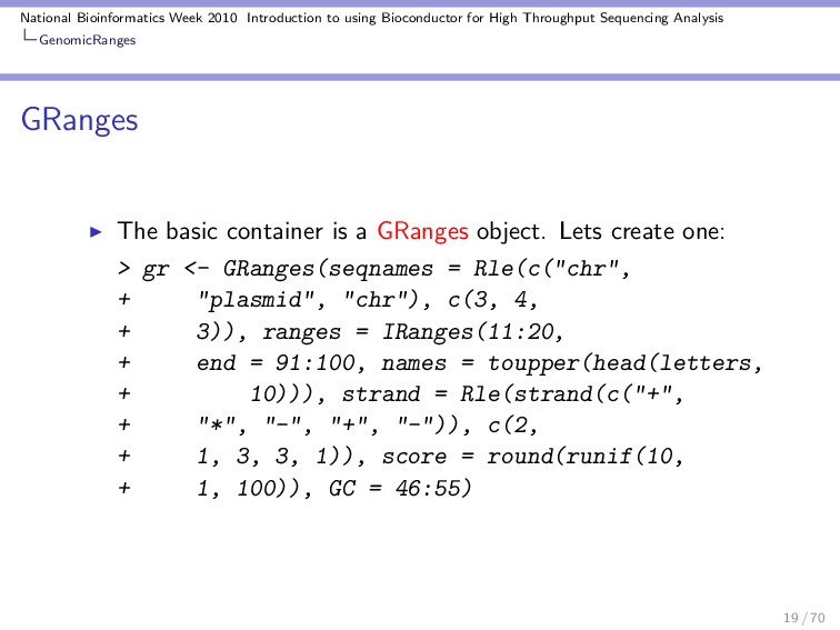
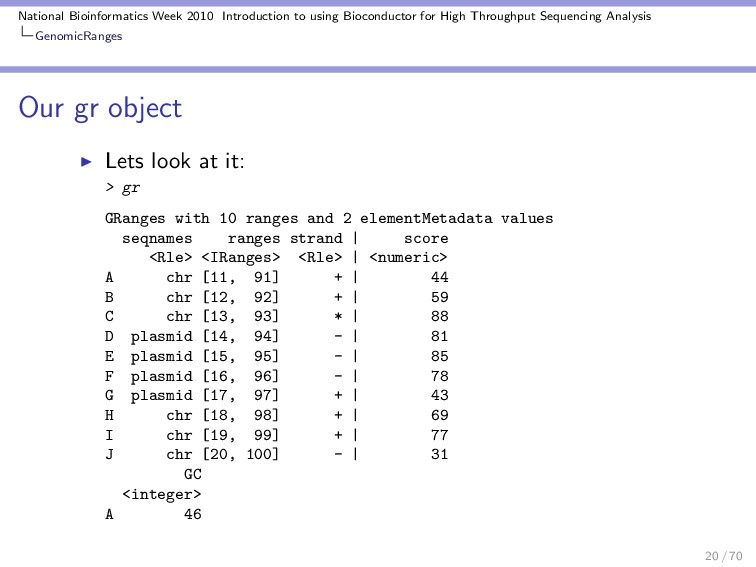
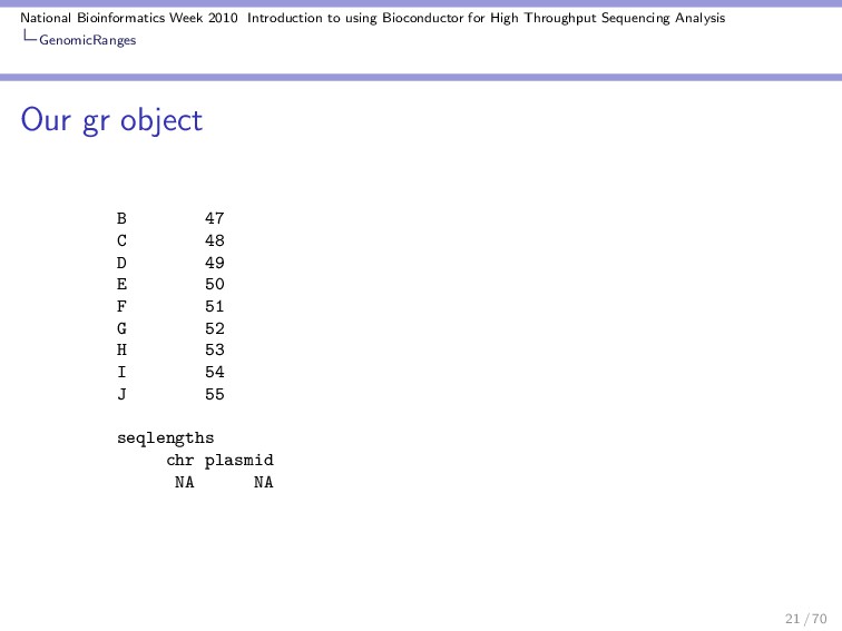
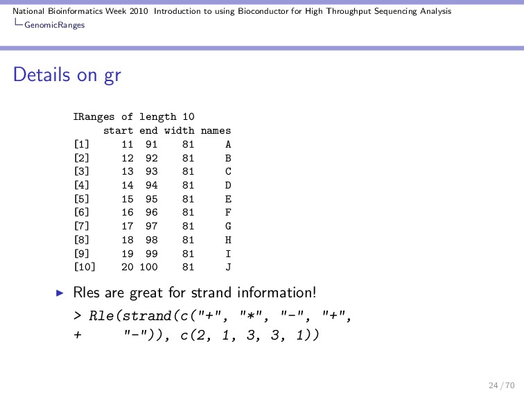
19. National Bioinformatics Week 2010 Introduction to using Bioconductor for High Throughput Sequencing Analysis GenomicRanges GRanges The basic container is a GRanges object. Lets create one: > gr <- GRanges(seqnames = Rle(c("chr", + "plasmid", "chr"), c(3, 4, + 3)), ranges = IRanges(11:20, + end = 91:100, names = toupper(head(letters, + 10))), strand = Rle(strand(c("+", + "*", "-", "+", "-")), c(2, + 1, 3, 3, 1)), score = round(runif(10, + 1, 100)), GC = 46:55) 19 / 70
20. National Bioinformatics Week 2010 Introduction to using Bioconductor for High Throughput Sequencing Analysis GenomicRanges Our gr object Lets look at it: > gr GRanges with 10 ranges and 2 elementMetadata values seqnames ranges strand | score <Rle> <IRanges> <Rle> | <numeric> A chr [11, 91] + | 44 B chr [12, 92] + | 59 C chr [13, 93] * | 88 D plasmid [14, 94] - | 81 E plasmid [15, 95] - | 85 F plasmid [16, 96] - | 78 G plasmid [17, 97] + | 43 H chr [18, 98] + | 69 I chr [19, 99] + | 77 J chr [20, 100] - | 31 GC <integer> A 46 20 / 70
21. National Bioinformatics Week 2010 Introduction to using Bioconductor for High Throughput Sequencing Analysis GenomicRanges Our gr object B 47 C 48 D 49 E 50 F 51 G 52 H 53 I 54 J 55 seqlengths chr plasmid NA NA 21 / 70
22. National Bioinformatics Week 2010 Introduction to using Bioconductor for High Throughput Sequencing Analysis GenomicRanges Details on gr Woah! Lots of info! Lets look at gr object a bit closer Yes, gr is a GRanges object > class(gr) [1] "GRanges" attr(,"package") [1] "GenomicRanges" An Run length encoded object (Rle) is useful when you repeat values. > Rle(c("chr", "plasmid", "chr"), + c(3, 4, 3)) 22 / 70
23. National Bioinformatics Week 2010 Introduction to using Bioconductor for High Throughput Sequencing Analysis GenomicRanges Details on gr 'character' Rle of length 10 with 3 runs Lengths: 3 4 3 Values : "chr" "plasmid" "chr" Let’s look at how we made the IRanges object inside gr > head(letters, 2) [1] "a" "b" > toupper(head(letters, 2)) [1] "A" "B" > IRanges(11:20, end = 91:100, names = toupper(head(letters, + 10))) 23 / 70
24. National Bioinformatics Week 2010 Introduction to using Bioconductor for High Throughput Sequencing Analysis GenomicRanges Details on gr IRanges of length 10 start end width names [1] 11 91 81 A [2] 12 92 81 B [3] 13 93 81 C [4] 14 94 81 D [5] 15 95 81 E [6] 16 96 81 F [7] 17 97 81 G [8] 18 98 81 H [9] 19 99 81 I [10] 20 100 81 J Rles are great for strand information! > Rle(strand(c("+", "*", "-", "+", + "-")), c(2, 1, 3, 3, 1)) 24 / 70
25. National Bioinformatics Week 2010 Introduction to using Bioconductor for High Throughput Sequencing Analysis GenomicRanges Details on gr 'factor' Rle of length 10 with 5 runs Lengths: 2 1 3 3 1 Values : + * - + - Levels(3): + - * > round(runif(10, 1, 100)) [1] 23 52 71 77 60 1 47 6 76 10 > 46:55 [1] 46 47 48 49 50 51 52 53 54 55 25 / 70
26. National Bioinformatics Week 2010 Introduction to using Bioconductor for High Throughput Sequencing Analysis GenomicRanges Data extractors Once we have a GRanges we can extract subsets of the informations: Replicon names: > seqnames(gr) 'factor' Rle of length 10 with 3 runs Lengths: 3 4 3 Values : chr plasmid chr Levels(2): chr plasmid The actual ranges: > ranges(gr) 26 / 70
27. National Bioinformatics Week 2010 Introduction to using Bioconductor for High Throughput Sequencing Analysis GenomicRanges Data extractors IRanges of length 10 start end width names [1] 11 91 81 A [2] 12 92 81 B [3] 13 93 81 C [4] 14 94 81 D [5] 15 95 81 E [6] 16 96 81 F [7] 17 97 81 G [8] 18 98 81 H [9] 19 99 81 I [10] 20 100 81 J Strand info: 27 / 70
28. National Bioinformatics Week 2010 Introduction to using Bioconductor for High Throughput Sequencing Analysis GenomicRanges Data extractors > strand(gr) 'factor' Rle of length 10 with 5 runs Lengths: 2 1 3 3 1 Values : + * - + - Levels(3): + - * Specific custom variables: > values(gr)[, "GC"] [1] 46 47 48 49 50 51 52 53 54 55 Ranges names: > names(gr) [1] "A" "B" "C" "D" "E" "F" "G" "H" "I" [10] "J" 28 / 70
29. National Bioinformatics Week 2010 Introduction to using Bioconductor for High Throughput Sequencing Analysis GenomicRanges Data extractors The total number of ranges: > length(gr) [1] 10 Modify the length of the replicons: > seqlengths(gr) <- c(4e+06, 1e+05) Length of the ranges: > width(gr) [1] 81 81 81 81 81 81 81 81 81 81 29 / 70
30. National Bioinformatics Week 2010 Introduction to using Bioconductor for High Throughput Sequencing Analysis GenomicRanges Manipulating GRanges These are some useful functions / operations for manipulating a GRanges object: Divide into several objects: > split(gr) GRangesList of length 10 $A GRanges with 1 range and 2 elementMetadata values seqnames ranges strand | score <Rle> <IRanges> <Rle> | <numeric> A chr [11, 91] + | 44 GC <integer> A 46 $B GRanges with 1 range and 2 elementMetadata values seqnames ranges strand | score <Rle> <IRanges> <Rle> | <numeric> 30 / 70
31. National Bioinformatics Week 2010 Introduction to using Bioconductor for High Throughput Sequencing Analysis GenomicRanges Manipulating GRanges B chr [12, 92] + | 59 GC <integer> B 47 $C GRanges with 1 range and 2 elementMetadata values seqnames ranges strand | score <Rle> <IRanges> <Rle> | <numeric> C chr [13, 93] * | 88 GC <integer> C 48 ... <7 more elements> seqlengths 31 / 70
32. National Bioinformatics Week 2010 Introduction to using Bioconductor for High Throughput Sequencing Analysis GenomicRanges Manipulating GRanges chr plasmid 4000000 100000 > split(gr)[[9]] GRanges with 1 range and 2 elementMetadata values seqnames ranges strand | score <Rle> <IRanges> <Rle> | <numeric> I chr [19, 99] + | 77 GC <integer> I 54 seqlengths chr plasmid 4000000 100000 Subset select ranges: > gr[1:2] 32 / 70
33. National Bioinformatics Week 2010 Introduction to using Bioconductor for High Throughput Sequencing Analysis GenomicRanges Manipulating GRanges GRanges with 2 ranges and 2 elementMetadata values seqnames ranges strand | score <Rle> <IRanges> <Rle> | <numeric> A chr [11, 91] + | 44 B chr [12, 92] + | 59 GC <integer> A 46 B 47 seqlengths chr plasmid 4000000 100000 Reverse: 33 / 70
34. National Bioinformatics Week 2010 Introduction to using Bioconductor for High Throughput Sequencing Analysis GenomicRanges Manipulating GRanges > rev(gr[1]) GRanges with 1 range and 2 elementMetadata values seqnames ranges strand | score <Rle> <IRanges> <Rle> | <numeric> A chr [11, 91] + | 44 GC <integer> A 46 seqlengths chr plasmid 4000000 100000 Get the upstream regions of our ranges: 34 / 70
35. National Bioinformatics Week 2010 Introduction to using Bioconductor for High Throughput Sequencing Analysis GenomicRanges Manipulating GRanges > flank(gr, 10)[1:2] GRanges with 2 ranges and 2 elementMetadata values seqnames ranges strand | score <Rle> <IRanges> <Rle> | <numeric> A chr [1, 10] + | 44 B chr [2, 11] + | 59 GC <integer> A 46 B 47 seqlengths chr plasmid 4000000 100000 35 / 70
36. National Bioinformatics Week 2010 Introduction to using Bioconductor for High Throughput Sequencing Analysis GenomicRanges Manipulating GRanges Move our ranges: > shift(gr, 5)[1:2] GRanges with 2 ranges and 2 elementMetadata values seqnames ranges strand | score <Rle> <IRanges> <Rle> | <numeric> A chr [16, 96] + | 44 B chr [17, 97] + | 59 GC <integer> A 46 B 47 seqlengths 36 / 70
37. National Bioinformatics Week 2010 Introduction to using Bioconductor for High Throughput Sequencing Analysis GenomicRanges Manipulating GRanges chr plasmid 4000000 100000 Resize them: > resize(gr, 1)[1:2] GRanges with 2 ranges and 2 elementMetadata values seqnames ranges strand | score <Rle> <IRanges> <Rle> | <numeric> A chr [11, 11] + | 44 B chr [12, 12] + | 59 GC <integer> A 46 B 47 37 / 70
38. National Bioinformatics Week 2010 Introduction to using Bioconductor for High Throughput Sequencing Analysis GenomicRanges Manipulating GRanges seqlengths chr plasmid 4000000 100000 Compact overlapping ranges: > reduce(gr) GRanges with 5 ranges and 0 elementMetadata values seqnames ranges strand | <Rle> <IRanges> <Rle> | [1] chr [11, 99] + | [2] chr [20, 100] - | [3] chr [13, 93] * | [4] plasmid [17, 97] + | 38 / 70
39. National Bioinformatics Week 2010 Introduction to using Bioconductor for High Throughput Sequencing Analysis GenomicRanges Manipulating GRanges [5] plasmid [14, 96] - | seqlengths chr plasmid 4000000 100000 Find the gaps: > gaps(gr)[1:2] GRanges with 2 ranges and 0 elementMetadata values seqnames ranges strand | <Rle> <IRanges> <Rle> | [1] chr [ 1, 10] + | [2] chr [100, 4000000] + | 39 / 70
40. National Bioinformatics Week 2010 Introduction to using Bioconductor for High Throughput Sequencing Analysis GenomicRanges Manipulating GRanges seqlengths chr plasmid 4000000 100000 And most importantly, find the coverage! > coverage(gr) SimpleRleList of length 2 $chr 'integer' Rle of length 4000000 with 13 runs Lengths: 10 1 ... 3999900 Values : 0 1 ... 0 $plasmid 'integer' Rle of length 100000 with 9 runs 40 / 70
41. National Bioinformatics Week 2010 Introduction to using Bioconductor for High Throughput Sequencing Analysis GenomicRanges Manipulating GRanges Lengths: 13 1 ... 1 99903 Values : 0 1 ... 1 0 41 / 70
42. National Bioinformatics Week 2010 Introduction to using Bioconductor for High Throughput Sequencing Analysis Rsamtools BioC I/O packages ShortRead was the first one for HTS data. It’s great for reading Illumina output files (export, fastq), alignments from short read aligners such as Bowtie, Eland, . . . .3 With the surge of short read aligners, a group decided to create a unified format. The SAM format: http://samtools.sourceforge.net/ The format is detailed at http://samtools.sourceforge.net/SAM1.pdf and Rsamtools is the BioC package. Basically most tools now use the SAM format and its brother, the BAM format (binary files, less HD space!). Caveats. . . 3Definitely check the qa function if you use ShortRead! 42 / 70
43. National Bioinformatics Week 2010 Introduction to using Bioconductor for High Throughput Sequencing Analysis Rsamtools scanBAM scanBAM is the main function in this package! To read in a file you need to specify some parameters. For example, data from select ranges. Lets look at the example: > library(Rsamtools) > which <- RangesList(seq1 = IRanges(1000, + 2000), seq2 = IRanges(c(100, + 1000), c(1000, 2000))) > what <- c("rname", "strand", "pos", + "qwidth", "seq") > param <- ScanBamParam(which = which, + what = what) 43 / 70
44. National Bioinformatics Week 2010 Introduction to using Bioconductor for High Throughput Sequencing Analysis Rsamtools scanBAM Now we have all the pieces we need to read in a BAM file. Lets add the file path. > which SimpleRangesList of length 2 $seq1 IRanges of length 1 start end width [1] 1000 2000 1001 $seq2 IRanges of length 2 start end width [1] 100 1000 901 [2] 1000 2000 1001 44 / 70
45. National Bioinformatics Week 2010 Introduction to using Bioconductor for High Throughput Sequencing Analysis Rsamtools scanBAM > bamFile <- system.file("extdata", + "ex1.bam", package = "Rsamtools") And finally read the BAM file: > bam <- scanBam(bamFile, param = param) 45 / 70
46. National Bioinformatics Week 2010 Introduction to using Bioconductor for High Throughput Sequencing Analysis Rsamtools Understanding our bam object Careful! Don’t print the bam object since it is actually a list: > class(bam) [1] "list" > names(bam) [1] "seq1:1000-2000" "seq2:100-1000" [3] "seq2:1000-2000" In the list, we have one element per each range we specified. Each of those elements is another list: > class(bam[[1]]) [1] "list" > names(bam[[1]]) 46 / 70
47. National Bioinformatics Week 2010 Introduction to using Bioconductor for High Throughput Sequencing Analysis Rsamtools Understanding our bam object [1] "rname" "strand" "pos" "qwidth" [5] "seq" As we can see, we have one element per every variable we read in (specified in our what object). > sapply(bam[[1]], class) rname strand "factor" "factor" pos qwidth "integer" "integer" seq "DNAStringSet" 47 / 70
48. National Bioinformatics Week 2010 Introduction to using Bioconductor for High Throughput Sequencing Analysis Rsamtools To a DataFrame Probably an easier to use class is the DataFrame4 The transformation involves more complicated code: > lst <- lapply(names(bam[[1]]), + function(elt) { + do.call(c, unname(lapply(bam, + "[[", elt))) + }) > names(lst) <- names(bam[[1]]) > df <- do.call("DataFrame", lst) > head(df, 2) 48 / 70
49. National Bioinformatics Week 2010 Introduction to using Bioconductor for High Throughput Sequencing Analysis Rsamtools To a DataFrame DataFrame with 2 rows and 5 columns rname strand pos <integer> <integer> <integer> 1 1 1 970 2 1 1 971 qwidth <integer> 1 35 2 35 seq <DNAStringSet> 1 TATTAGGAAATGCTTTACTGTCATAACTATGAAGA 2 ATTAGGAAATGCTTTACTGTCATAACTATGAAGAG 4It isn’t a data.frame!!! 49 / 70
50. National Bioinformatics Week 2010 Introduction to using Bioconductor for High Throughput Sequencing Analysis Rsamtools THE advantage of BAM files BAM files are not only binary files, but they are indexed. Meaning that we can quickly read a subset of our aligned data! If you set na19240url to ftp://ftp-trace.ncbi.nih.gov/1000genomes/ftp/ pilot_data/data/NA19240/alignment/NA19240.chrom6. SLX.maq.SRP000032.2009_07.bam you can do the reading the following data subset: > which <- GRanges(seqnames = "6", + ranges = IRanges(1e+05, 110000)) > param <- ScanBamParam(which = which) > na19240bam <- scanBam(na19240url, + param = param) 50 / 70
51. National Bioinformatics Week 2010 Introduction to using Bioconductor for High Throughput Sequencing Analysis Rsamtools THE advantage of BAM files Rsamtools also includes functions for dealing with multiple BAM files. 51 / 70
52. National Bioinformatics Week 2010 Introduction to using Bioconductor for High Throughput Sequencing Analysis ChIPpeakAnno Overview It’s one of the newest packages for ChIP-seq workflows. It integrates functionality across several packages. Basic idea: compare a set of ranges with annotation ranges, find the closest ones and make tests. I find it to be a very interesting tool box :) 52 / 70
53. National Bioinformatics Week 2010 Introduction to using Bioconductor for High Throughput Sequencing Analysis ChIPpeakAnno A quick demo Lets load the example data: > library(ChIPpeakAnno) > data(myPeakList) > data(TSS.human.GRCh37) > head(myPeakList, 2) RangedData with 2 rows and 0 value columns across 24 spaces space <character> 1_93_556427 1 1_41_559455 1 ranges | <IRanges> | 1_93_556427 [556660, 556760] | 1_41_559455 [559774, 559874] | > head(TSS.human.GRCh37, 2) 53 / 70
54. National Bioinformatics Week 2010 Introduction to using Bioconductor for High Throughput Sequencing Analysis ChIPpeakAnno A quick demo RangedData with 2 rows and 2 value columns across 72 spaces space <character> ENSG00000223972 1 ENSG00000227232 1 ranges | <IRanges> | ENSG00000223972 [11874, 14412] | ENSG00000227232 [14363, 29570] | strand <integer> ENSG00000223972 1 ENSG00000227232 -1 ENSG00000223972 DEAD/H (Asp-Glu-Ala-Asp/His) box polypeptide 11 like 10 [S ENSG00000227232 WAS protein family homolog 5 pseudogene [S Using annotatePeakInBatch we can associate the two types of ranges: 54 / 70
55. National Bioinformatics Week 2010 Introduction to using Bioconductor for High Throughput Sequencing Analysis ChIPpeakAnno A quick demo > annotatedPeak = annotatePeakInBatch(myPeakList[1:6, + ], AnnotationData = TSS.human.GRCh37) > head(annotatedPeak, 2) RangedData with 2 rows and 9 value columns across 1 space space <character> 1_14_1269014 ENSG00000169962 1 1_11_1041174 ENSG00000131591 1 ranges <IRanges> 1_14_1269014 ENSG00000169962 [1270239, 1270339] 1_11_1041174 ENSG00000131591 [1041646, 1041746] | | 1_14_1269014 ENSG00000169962 | 1_11_1041174 ENSG00000131591 | peak <character> 1_14_1269014 ENSG00000169962 1_14_1269014 55 / 70
56. National Bioinformatics Week 2010 Introduction to using Bioconductor for High Throughput Sequencing Analysis ChIPpeakAnno A quick demo 1_11_1041174 ENSG00000131591 1_11_1041174 strand <character> 1_14_1269014 ENSG00000169962 1 1_11_1041174 ENSG00000131591 -1 feature <character> 1_14_1269014 ENSG00000169962 ENSG00000169962 1_11_1041174 ENSG00000131591 ENSG00000131591 start_position <numeric> 1_14_1269014 ENSG00000169962 1266694 1_11_1041174 ENSG00000131591 1017198 end_position <numeric> 1_14_1269014 ENSG00000169962 1270686 1_11_1041174 ENSG00000131591 1051741 insideFeature <character> 1_14_1269014 ENSG00000169962 inside 56 / 70
57. National Bioinformatics Week 2010 Introduction to using Bioconductor for High Throughput Sequencing Analysis ChIPpeakAnno A quick demo 1_11_1041174 ENSG00000131591 inside distancetoFeature <numeric> 1_14_1269014 ENSG00000169962 3545 1_11_1041174 ENSG00000131591 10095 shortestDistance <numeric> 1_14_1269014 ENSG00000169962 347 1_11_1041174 ENSG00000131591 9995 fromOverlappingOrNearest <character> 1_14_1269014 ENSG00000169962 NearestStart 1_11_1041174 ENSG00000131591 NearestStart Export to Excel5 > write.table(as.data.frame(annotatedPeak), + file = "annotatedPeakList.xls", + sep = "\t", row.names = FALSE) 5Though it might be faster to manipulate in R :) 57 / 70
58. National Bioinformatics Week 2010 Introduction to using Bioconductor for High Throughput Sequencing Analysis ChIPpeakAnno Peak distribution distance to your annotation > y = annotatedPeak$distancetoFeature[!is.na(annotatedPeak$distancetoFeature) & + annotatedPeak$fromOverlappingOrNearest == + "NearestStart"] > hist(y, xlab = "Distance To Nearest TSS", + main = "", breaks = 1000, xlim = c(min(y) - + 100, max(y) + 100)) 58 / 70
59. National Bioinformatics Week 2010 Introduction to using Bioconductor for High Throughput Sequencing Analysis ChIPpeakAnno Peak distribution distance to your annotation Distance To Nearest TSS Frequency −5000 0 5000 10000 0.0 0.2 0.4 0.6 0.8 1.0 59 / 70
60. National Bioinformatics Week 2010 Introduction to using Bioconductor for High Throughput Sequencing Analysis ChIPpeakAnno And a look at the genomic regions > temp = as.data.frame(annotatedPeak) > pie(table(temp[as.character(temp$fromOverlappingOrNearest) == + "Overlapping" | (as.character(temp$fromOverlappingOrNearest) == + "NearestStart" & !temp$peak %in% + temp[as.character(temp$fromOverlappingOrNearest) == + "Overlapping", ]$peak), + ]$insideFeature)) 60 / 70
61. National Bioinformatics Week 2010 Introduction to using Bioconductor for High Throughput Sequencing Analysis ChIPpeakAnno And a look at the genomic regions downstream inside upstream 61 / 70
62. National Bioinformatics Week 2010 Introduction to using Bioconductor for High Throughput Sequencing Analysis ChIPpeakAnno A second example Say that you have 3 replicates and you want to check how significant is the overlap between the peaks and visualize it as a Venn diagram. Lets load the example data. > data(Peaks.Ste12.Replicate1) > data(Peaks.Ste12.Replicate2) > data(Peaks.Ste12.Replicate3) > head(Peaks.Ste12.Replicate1, 2) 62 / 70
63. National Bioinformatics Week 2010 Introduction to using Bioconductor for High Throughput Sequencing Analysis ChIPpeakAnno A second example RangedData with 2 rows and 1 value column across 16 spa space ranges | <character> <IRanges> | 22 chr1 [67961, 70254] | 23 chr1 [67961, 70254] | strand <integer> 22 1 23 1 63 / 70
64. National Bioinformatics Week 2010 Introduction to using Bioconductor for High Throughput Sequencing Analysis ChIPpeakAnno Venn diagram > makeVennDiagram(RangedDataList(Peaks.Ste12.Replicate1, + Peaks.Ste12.Replicate2, Peaks.Ste12.Replicate3), + NameOfPeaks = c("Replicate1", + "Replicate2", "Replicate3"), + maxgap = 0, totalTest = 1580) $p.value.1vs2 [1] 6.803956e-91 $p.value.1vs3 [1] 4.54906e-107 $p.value.2vs3 [1] 1.853842e-85 $vennCounts Replicate1 Replicate2 Replicate3 [1,] 0 0 0 [2,] 0 0 1 [3,] 0 1 0 64 / 70
65. National Bioinformatics Week 2010 Introduction to using Bioconductor for High Throughput Sequencing Analysis ChIPpeakAnno Venn diagram [4,] 0 1 1 [5,] 1 0 0 [6,] 1 0 1 [7,] 1 1 0 [8,] 1 1 1 Counts [1,] 589 [2,] 72 [3,] 189 [4,] 470 [5,] 103 [6,] 453 [7,] 520 [8,] 408 attr(,"class") [1] "VennCounts" 65 / 70
66. National Bioinformatics Week 2010 Introduction to using Bioconductor for High Throughput Sequencing Analysis ChIPpeakAnno Venn diagram Replicate1 Replicate2 Replicate3 589 72 189 470 103 453 520 408 66 / 70
67. National Bioinformatics Week 2010 Introduction to using Bioconductor for High Throughput Sequencing Analysis ChIPpeakAnno Other useful tools BED / GFF import Get annotation from a public database using biomaRt Get the sequences nearby interesting peaks to do motif discovery Get GO terms and test for significant enrichment Find the peak distance to other features in custom ways. 67 / 70
68. National Bioinformatics Week 2010 Introduction to using Bioconductor for High Throughput Sequencing Analysis ChIPpeakAnno Session Information > sessionInfo() R version 2.11.1 (2010-05-31) x86_64-pc-linux-gnu locale: [1] LC_CTYPE=en_US.utf8 [2] LC_NUMERIC=C [3] LC_TIME=en_US.utf8 [4] LC_COLLATE=en_US.utf8 [5] LC_MONETARY=C [6] LC_MESSAGES=en_US.utf8 [7] LC_PAPER=en_US.utf8 [8] LC_NAME=C [9] LC_ADDRESS=C [10] LC_TELEPHONE=C [11] LC_MEASUREMENT=en_US.utf8 [12] LC_IDENTIFICATION=C attached base packages: 68 / 70
69. National Bioinformatics Week 2010 Introduction to using Bioconductor for High Throughput Sequencing Analysis ChIPpeakAnno Session Information [1] stats graphics grDevices [4] utils datasets methods [7] base other attached packages: [1] ChIPpeakAnno_1.4.1 [2] limma_3.4.4 [3] org.Hs.eg.db_2.4.1 [4] GO.db_2.4.1 [5] RSQLite_0.9-2 [6] DBI_0.2-5 [7] AnnotationDbi_1.10.2 [8] BSgenome.Ecoli.NCBI.20080805_1.3.16 [9] BSgenome_1.16.5 [10] multtest_2.5.14 [11] Biobase_2.8.0 [12] biomaRt_2.4.0 [13] Rsamtools_1.0.7 [14] Biostrings_2.16.9 [15] GenomicRanges_1.0.7 69 / 70
70. National Bioinformatics Week 2010 Introduction to using Bioconductor for High Throughput Sequencing Analysis ChIPpeakAnno Session Information [16] IRanges_1.6.11 loaded via a namespace (and not attached): [1] MASS_7.3-7 RCurl_1.4-3 [3] splines_2.11.1 survival_2.35-8 [5] tools_2.11.1 XML_3.1-0 70 / 70