fergus_deblurring.pdf

Transcript

1. Removing Camera Shake from Removing Camera Shake from a Single Photograph Rob Fergus, Barun Singh, Aaron Hertzmann, Sam T. Roweis and William T. Freeman Massachusetts Institute of Technology gy and University of Toronto
2. Overview Joint work with B. Singh, A. Hertzmann, S.T. Roweis & W.T. Freeman Original Our algorithm
3. Close-up Original Naïve sharpening Our algorithm
4. Let’s take a photo Blurry result
5. Slow-motion replay
6. Slow-motion replay Motion of camera
7. Image formation process = ⊗ Bl Blurry image Sharp image Blur kernel Input to algorithm Desired output Convolution operator Model is approximation Assume static scene
8. Existing work on image deblurring Old problem: – Trott, T., “The Effect of Motion of Resolution”, Photogrammetric Engineering, Vol. 26, pp. 819-827, 1960. – Slepian, D., “Restoration of Photographs Blurred by Image Motion”, Bell System Tech., Vol. 46, No. 10, pp. 2353-2362, 1967.
9. Existing work on image deblurring Software algorithms for natural images – Many require multiple images – Mainly Fourier and/or Wavelet based Mainly Fourier and/or Wavelet based – Strong assumptions about blur Æ not true for camera shake Æ not true for camera shake Assumed forms of blur kernels – Image constraints are frequency-domain power-laws
10. Existing work on image deblurring Hardware approaches Dual cameras Coded shutter Image stabilizers Ben-Ezra & Nayar CVPR 2004 Raskar et al. SIGGRAPH 2006 Our approach can be combined with these hardware methods
11. Why is this hard? Simple analogy: 11 is the product of two numbers. What are they? No unique solution: 11 = 1 x 11 11 = 1 x 11 11 = 2 x 5.5 11 3 3 667 11 = 3 x 3.667 etc….. Need more information !!!!
12. Multiple possible solutions Sharp image Blur kernel = ⊗ Blurry image = ⊗ = ⊗
13. Natural image statistics Characteristic distribution with heavy tails Histogram of image gradients els Log # pixe
14. Blurry images have different statistics Histogram of image gradients els Log # pixe
15. Parametric distribution Histogram of image gradients els Log # pixe Use parametric model of sharp image statistics
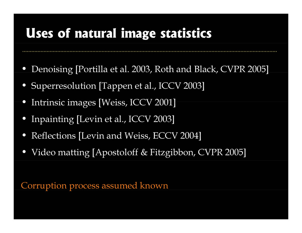
16. Uses of natural image statistics • Denoising [Portilla et al. 2003, Roth and Black, CVPR 2005] g [ , , ] • Superresolution [Tappen et al., ICCV 2003] • Intrinsic images [Weiss ICCV 2001] • Intrinsic images [Weiss, ICCV 2001] • Inpainting [Levin et al., ICCV 2003] • Reflections [Levin and Weiss, ECCV 2004] • Video matting [Apostoloff & Fitzgibbon, CVPR 2005] Corruption process assumed known p p
17. Three sources of information 1. Reconstruction constraint: ⊗ = ⊗ Estimated Input blurry image Estimated sharp image Estimated blur kernel 2 I i 3 Blur prior: 2. Image prior: 3. Blur prior: Positive Di ib i & Sparse Distribution of gradients
18. Three sources of information y = observed image b = blur kernel x = sharp image
19. Three sources of information y = observed image b = blur kernel x = sharp image p(b, x|y) Posterior p( , |y)
20. Three sources of information y = observed image b = blur kernel x = sharp image p(b, x|y) = k p(y|b, x) p(x) p(b) Posterior 1. Likelihood (Reconstruction t i t) 2. Image prior 3. Blur prior p( , |y) p(y| , ) p( ) p( ) constraint)
21. 1. Likelihood p(y|b, x) y = observed image b = blur x = sharp image Reconstruction constraint: ( |b ) N( | b 2) (x ⊗b y )2 p(y|b, x) = i N(yi |xi ⊗ b, σ2) ∝ i e −(xi⊗b−yi)2 2σ2 i - pixel index
22. 2. Image prior p(x) y = observed image b = blur x = sharp image p(x) = Q i PC c=1 πc N(f(xi)|0, s2 c ) Mixture of Gaussians fit to l d b f empirical distribution of image gradients pixels i - pixel index i i d Log # p c - mixture component index f - derivative filter
23. 3. Blur prior p(b) y = observed image b = blur x = sharp image p(b) = Q j PD d=1 πd E(bj|λd) Mixture of Exponentials 60 70 Most elements near zero – Positive & sparse – No connectivity constraint 40 50 p(b) Most elements near zero j blur kernel element y 10 20 30 A few can be large j - blur kernel element d - mixture component index 0 0.01 0.02 0.03 0.04 0.05 0.06 0.07 0.08 0.09 0.1 0 b
24. The obvious thing to do p(b, x|y) = k p(y|b, x) p(x) p(b) Posterior 1. Likelihood (Reconstruction constraint) 2. Image prior 3. Blur prior – Combine 3 terms into an objective function ) – Run conjugate gradient descent – This is Maximum a-Posteriori (MAP) ( ) No success!
25. Variational Bayesian approach Keeps track of uncertainty in estimates of image and blur by p y g y using a distribution instead of a single estimate Optimization surface for a single variable single variable Maximum a-Posteriori (MAP) re Variational Bayes Scor y Pixel intensity
26. Variational Independent Component Analysis Miskin and Mackay 2000 • Binary images Miskin and Mackay, 2000 y g • Priors on intensities • Small, synthetic blurs • Not applicable to pp natural images
27. Setup of Variational Approach Work in gradient domain: → ∇x ⊗ b = ∇y x ⊗ b = y A i i (∇ b|∇ ) Approximate posterior with p(∇x, b|∇y) q(∇x, b) is Gaussian on each pixel q(∇x, b) = q(∇x)q(b) q(∇x) Assume is Gaussian on each pixel is rectified Gaussian on each blur kernel element q(∇ ) q(b) KL(q(∇x)q(b) || p(∇x, b|∇y)) Cost function
28. Overview of algorithm Input image p g 1. Pre-processing 2. Kernel estimation - Multi-scale approach 3. Image reconstruction - Standard non-blind deconvolution routine
29. Preprocessing C t t Input image R Convert to grayscale Remove gamma correction User selects patch User selects patch from image B i i f Bayesian inference too slow to run on whole image g Infer kernel from this patch
30. Initialization Input image C t t R Convert to grayscale Remove gamma correction User selects patch User selects patch from image Initialize 3x3 blur kernel Initial blur kernel Blurry patch Initial image estimate
31. Inferring the kernel: multiscale method Input image C t t R Convert to grayscale Remove gamma correction User selects patch Loop over scales User selects patch from image Variational Bayes Upsample estimates Initialize 3x3 blur kernel Use multi-scale approach to avoid local minima:
32. Image Reconstruction Input image C t t R Convert to grayscale Remove gamma correction User selects patch Loop over scales User selects patch from image Full resolution blur estimate Variational Bayes Upsample estimates Initialize 3x3 blur kernel Non-blind deconvolution Deblurred (Richardson-Lucy) Deblurred image
33. Synthetic Synthetic experiments
34. Is blur kernel really stationary? 8 different people, handholding camera, using 1 second exposure
35. Dots from each corner Top Top Person 1 Person 2 Top left p right Bot. left Bot. right Person 3 Person 4
36. Synthetic example Sharp image Artificial blur trajectory 2 j y 4 6 8 0 2 4 6 8 0 2
37. Synthetic blurry image
38. Inference – initial scale Image before Image after Kernel before Kernel after Kernel before Kernel after
39. Inference – scale 2 Image before Image after Kernel before Kernel after Kernel before Kernel after
40. Inference – scale 3 Image before Image after Kernel before Kernel after Kernel before Kernel after
41. Inference – scale 4 Image before Image after Kernel before Kernel after Kernel before Kernel after
42. Inference – scale 5 Image before Image after Kernel before Kernel after Kernel before Kernel after
43. Inference – scale 6 Image before Image after Kernel before Kernel after Kernel before Kernel after
44. Inference – Final scale Image before Image after Kernel before Kernel after Kernel before Kernel after
45. Comparison of kernels 2 True kernel Estimated kernel 2 4 6 8 8 0 2 4 6 8 0 2
46. Blurry image
47. Matlab’s deconvblind
48. Blurry image
49. Our output
50. True sharp image
51. What we do and don’t model DO • Gamma correction • Tone response curve (if known) p ( ) DON’T • Saturation • Jpeg artifacts Jpeg artifacts • Scene motion • Color channel correlations • Color channel correlations
52. Real Real experiments
53. Results on real images Submitted by people from their own photo collections Type of camera unknown Output does contain artifacts – Increased noise – Ringing Compare with existing methods
54. Original photograph
55. Blur kernel Our output
56. Matlab’s deconvblind
57. Close-up Matlab’s Original Our output deconvblind
58. Original photograph
59. 2 4 6 Our output Blur kernel 6 8 2 4 6 8 10 12
60. Photoshop sharpen more
61. Original image Close up Close-up 2 4 6 8 2 4 6 8 10 12 Close-up of image Blur kernel Close-up of our output
62. Original photograph
63. Our output Blur kernel
64. Photoshop “Smart Sharpen” Blur kernel
65. Matlab’s deconvblind
66. Original photograph
67. 1 2 3 4 5 Our output 6 7 8 9 Blur kernel
68. Original photograph
69. Our output Blur kernel
70. Close-up of AV equipment Our output Original photograph
71. Original image
72. Our output Blur kernel
73. Close-up Blur kernel Our output Original image
74. What about a sharp image? Original photograph
75. 1 2 3 4 5 Our output 1 2 3 4 5 6 7 6 7 Blur kernel
78. Close-up • Original • Output p
79. Original photograph
80. Blur kernel Our output
81. Close-up Blur kernel O O i i l i Our output Original image
82. O i i l h t h Original photograph
83. Blurry image patch Our output Our output Blur kernel
84. Original photograph
85. Our output Blur kernel
86. Close-up of bird p Original Unsharp mask Our output O g a Unsharp mask Our output
87. Original photograph
88. Blur kernel Our output
89. Image artifacts & estimated kernels Blur kernels Image patterns Note: blur kernels were inferred from large image patches, NOT the image patterns shown
90. Code available online http://people.csail.mit.edu/fergus/research/deblur.html
91. Summary First method that can handle First method that can handle complicated real-world blur kernels Results still contain artifacts Big leap on an old, hard problem 2 4 6 8 0 Many things to improve: – Non-blind deconvolution, saturation etc. 2 4 6 8 10 12 14 16 18 20 2 4 6 8 0 ,
95. Gamma Digital image formation process Gamma correction RAW values Remapped values Blur process applied here P. Debevec & J. Malik, Recovering High Dynamic Range Radiance Maps from Photographs”, SIGGRAPH 97
96. Simple 1-D example y = bx + n y = observed image y = bx + n y = observed image b = blur x = sharp image x = sharp image n = noise N(0 σ2) n = noise ~ N(0,σ2) Let y = 2
97. p(b, x|y) = k p(y|b, x) p(x) p(b) Let y = 2 Let y = 2 σ2 = 0.1 N(y|bx, σ2) (y| , )
98. p(b, x|y) = k p(y|b, x) p(x) p(b) Gaussian distribution: Gaussian distribution: N(x|0, 2) N( | , )
99. p(b, x|y) = k p(y|b, x) p(x) p(b)
100. Marginal distribution p(b|y) p(b|y) = R p(b, x|y) dx = k R p(y|b, x) p(x) dx 0.14 0.16 0.1 0.12 b|y) 0.06 0.08 Bayes p(b 0.02 0.04 0 1 2 3 4 5 6 7 8 9 10 0 b
101. MAP solution Highest point on surface: argmaxb,x p(x, b|y) 0.14 0.16 0.1 0.12 b|y) 0.06 0.08 Bayes p(b 0.02 0.04 0 1 2 3 4 5 6 7 8 9 10 0 b
102. Variational Bayes • True Bayesian • True Bayesian approach not tractable tractable • Approximate posterior p with simple distribution
103. Fitting posterior with a Gaussian • Approximating distribution is Gaussian q(x, b) • Minimize KL(q(x, b) || p(x, b|y))
104. KL-Distance vs Gaussian width 10 11 9 10 8 (q||p) 7 KL( 5 6 0 0.1 0.2 0.3 0.4 0.5 0.6 0.7 4 Gaussian width
105. Variational Approximation of Marginal 2.5 2 Variational 1.5 y) True marginal 1 p(b|y MAP 0.5 0 1 2 3 4 5 6 7 8 9 10 0 b
106. Try sampling from the model Let true b = 2 0.8 0.9 1 R t 0 5 0.6 0.7 |y) Repeat: • Sample x ~ N(0,2) 0.3 0.4 0.5 p(b • Sample n ~ N(0,σ2) • y = xb + n 0 1 2 3 4 5 6 7 8 9 10 0 0.1 0.2 y xb n • Compute pMAP (b|y), pBayes (b|y) & pVariational (b|y) b • Multiply with existing density estimates (assume iid)
107. Original photograph
108. Our output 2 4 4 6 8 0 2 2 4 6 8 10 12 14 16 18 20 4 6 8 0 Blur kernel
109. Close-up of child Our output Original photograph