Anomaly Detection for Real-World Systems.

My talk on Anomaly Detection system and algorithms that I gave at DataEngConf NYC 2016.

Transcript

1. ANOMALY DETECTION FOR REAL-WORLD SYSTEMS Manojit Nandi Data Scientist STEALTHbits Technologies @mnandi92
2. WHAT ARE ANOMALIES? • Hard to define; “You’ll know it when you see it”. • Generally, anomalies are “anything that noticeably different” from the expected. • One important thing to keep in mind is that what is considered anomalous now may not be considered anomalous in the future.
3. Different approaches to anomaly detection • We can develop a statistical model of normal behavior. Then we can test how likely an observation is under the model. • We can take a machine learning approach and use a classifier to classify data points as “normal” or “anomalous”. • In this talk, I’m going to cover algorithms specially designed to detect anomalies. Photo Credit: Microsoft Azure
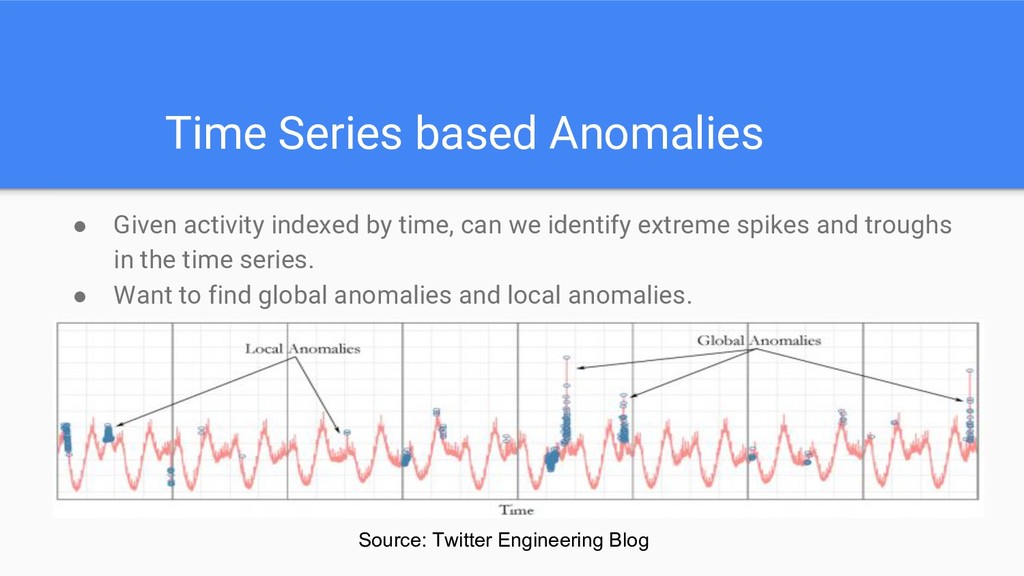
4. Anomalies in Data Streams • Problem: We have data streaming in continuously, and we want to identify anomalies in real-time. • Constraint: We can only examine the last 100 events in our sliding window. • In data streaming problems, we are “restricted” to quick-and-dirty methods due to the limited memory and need for rapid action.
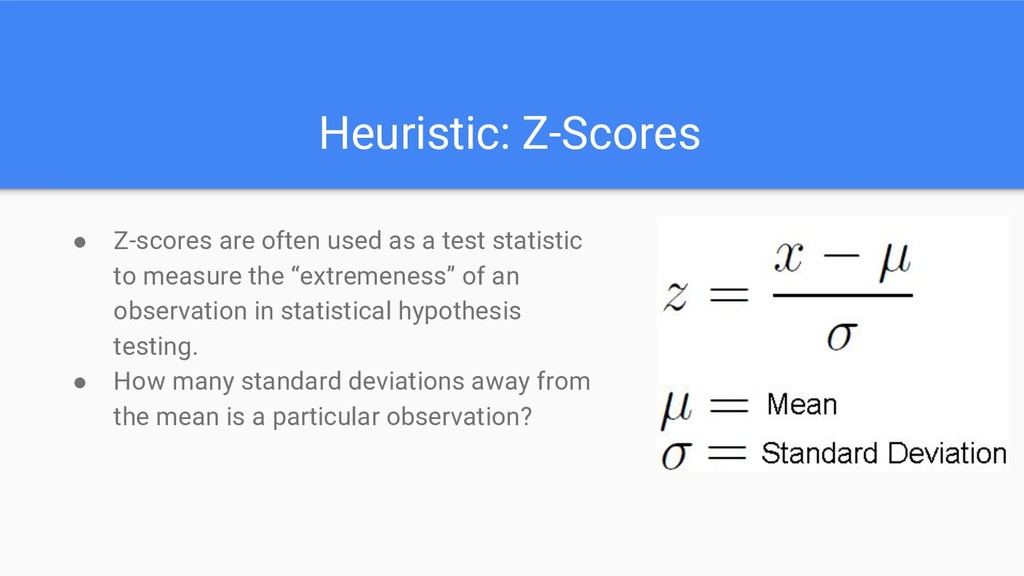
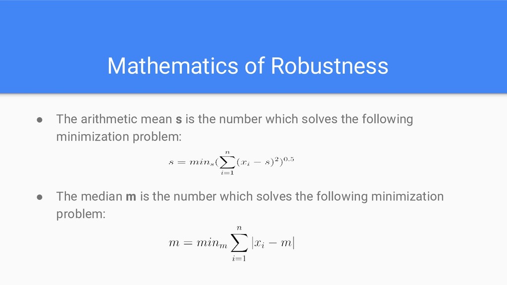
5. Heuristic: Z-Scores • Z-scores are often used as a test statistic to measure the “extremeness” of an observation in statistical hypothesis testing. • How many standard deviations away from the mean is a particular observation?
6. Moving Averages and Moving St. Dev. • As the data comes in, we keep track of the average and the standard deviation of the last n data points. • For each new data point, update the average and the standard deviation. • Using the new average and standard deviation, compute the z-score for this data point. • If the Z-score exceeds some threshold, flag the data point as anomalous.
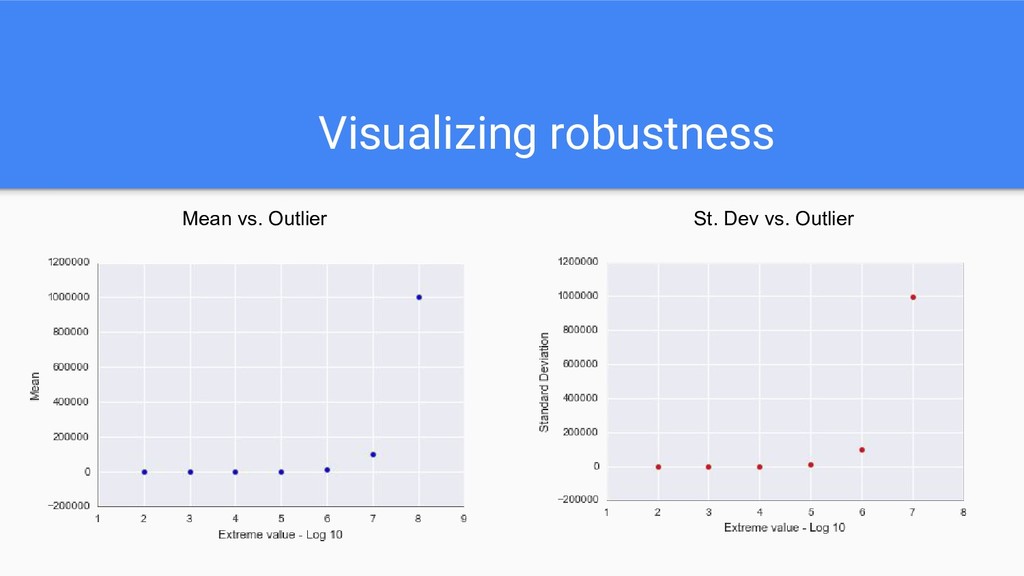
7. Standard Deviation not robust • Standard deviation (and mean, to a lesser extend) is highly sensitive to extreme values. • One extreme value can drastically increase the standard deviation. • As a result, the Z-scores for other data points dramatically decreases as well.
8. Mathematics of Robustness • The arithmetic mean s is the number which solves the following minimization problem: • The median m is the number which solves the following minimization problem:
9. Visualizing robustness Mean vs. Outlier St. Dev vs. Outlier
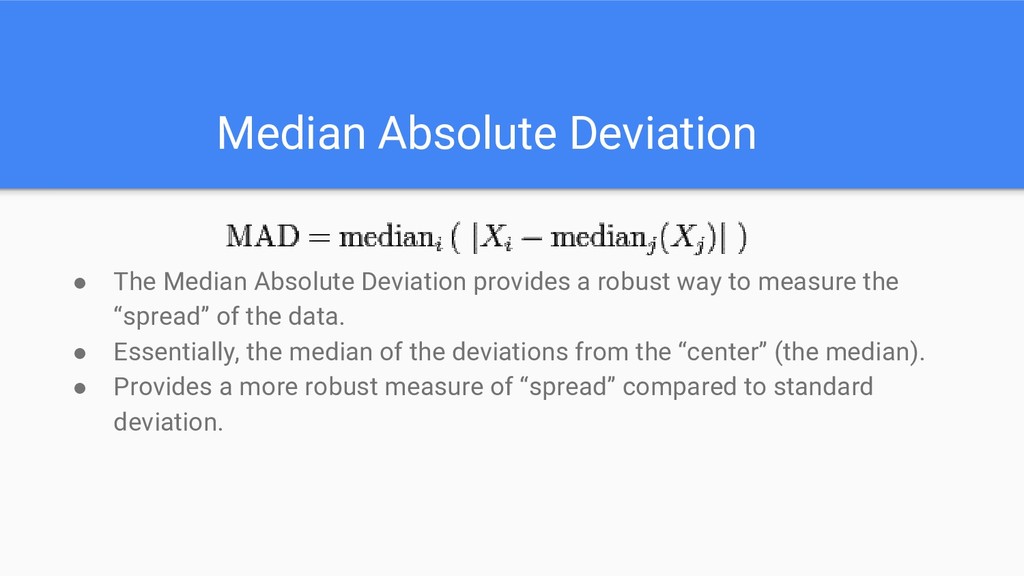
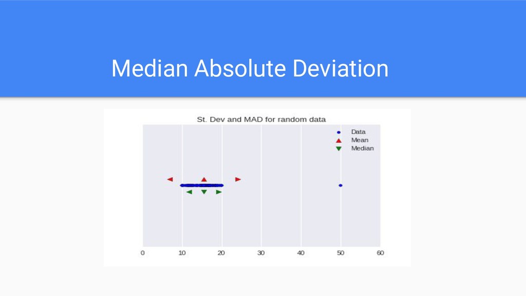
10. Median Absolute Deviation • The Median Absolute Deviation provides a robust way to measure the “spread” of the data. • Essentially, the median of the deviations from the “center” (the median). • Provides a more robust measure of “spread” compared to standard deviation.
11. Median Absolute Deviation
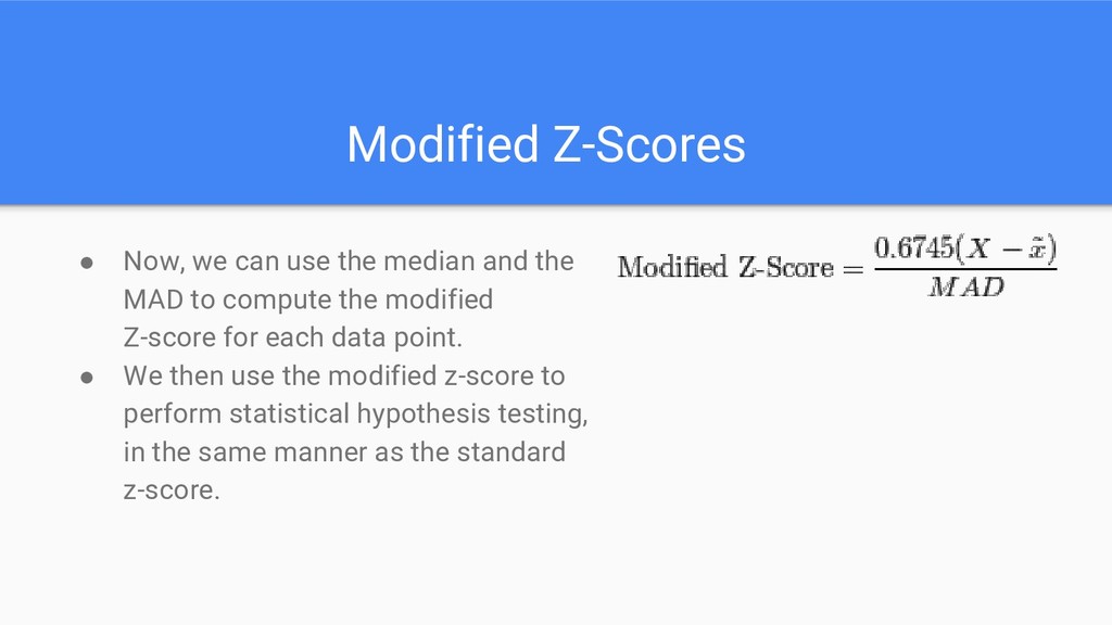
12. Modified Z-Scores • Now, we can use the median and the MAD to compute the modified Z-score for each data point. • We then use the modified z-score to perform statistical hypothesis testing, in the same manner as the standard z-score.
13. Density-Based Anomaly Detection • We have a bunch of points in some n-dimensional space. • Which ones are “noticeably” different from the others.
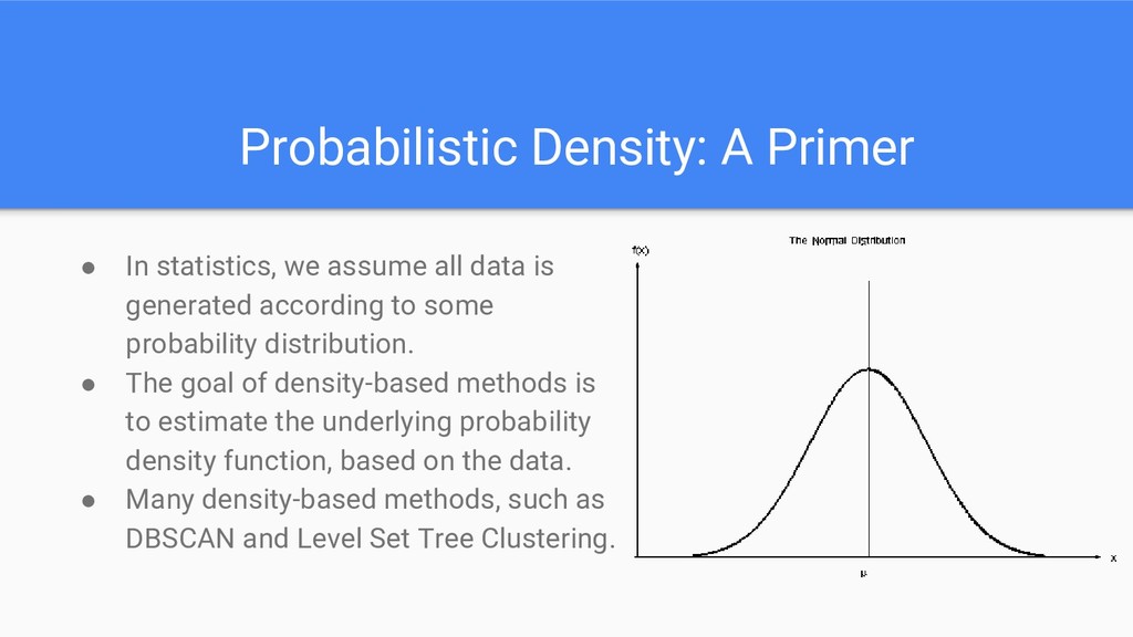
14. Probabilistic Density: A Primer • In statistics, we assume all data is generated according to some probability distribution. • The goal of density-based methods is to estimate the underlying probability density function, based on the data. • Many density-based methods, such as DBSCAN and Level Set Tree Clustering.
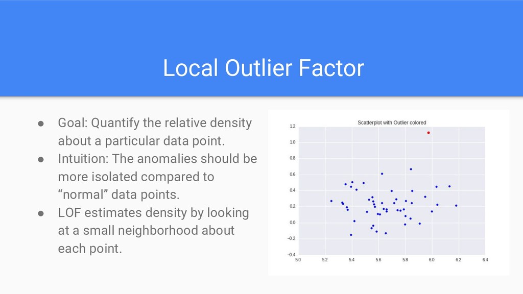
15. Local Outlier Factor • Goal: Quantify the relative density about a particular data point. • Intuition: The anomalies should be more isolated compared to “normal” data points. • LOF estimates density by looking at a small neighborhood about each point.
16. K-Distance • For each datapoint, compute the distance to the Kth-nearest neighbor. • Meta-heuristic: The K-distance gives us a notion of “volume”. • The more isolated a point is, the larger its k-distance.
17. Reachability Distance Reachability-Distance(A,B) = Max(K-Dist(B), Dist(A,B)) • “Do your close neighbors see you as one of their close neighbors”.
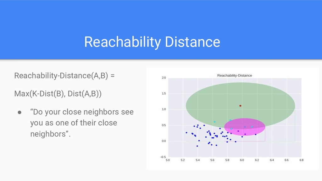
18. Local Reachability Density • Now, we are going to estimate the local density about each point. • For each data point, compute the average reachability-distance to its K-nearest neighbors. • The Local Reachability Density (LRD) of a data point A is defined as the inverse of this average reachability-distance.
19. Local Outlier Factor • LOF score is the ratio of point A’s density to the average density of its neighbors. • Outliers come from less dense areas, so the ratio is higher for outliers.
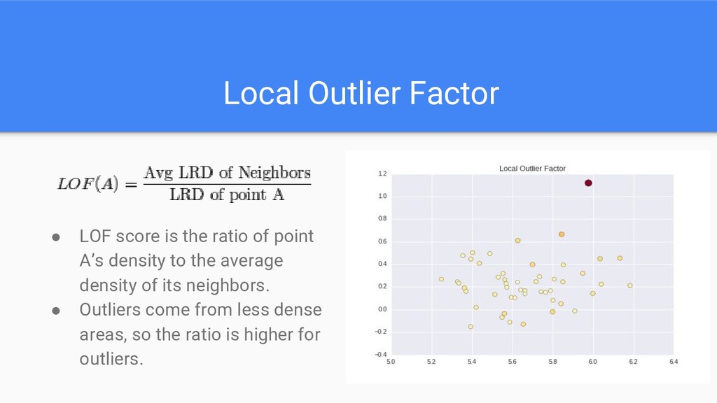
20. Interpreting LOF scores • Normal points have LOF scores between 1 and 1.5. • Anomalous points have much higher LOF scores. • If a point has a LOF score of 3, then this means the average density of this point’s neighbors is about 3x more dense than its local density.
21. Time Series based Anomalies • Given activity indexed by time, can we identify extreme spikes and troughs in the time series. • Want to find global anomalies and local anomalies. Source: Twitter Engineering Blog
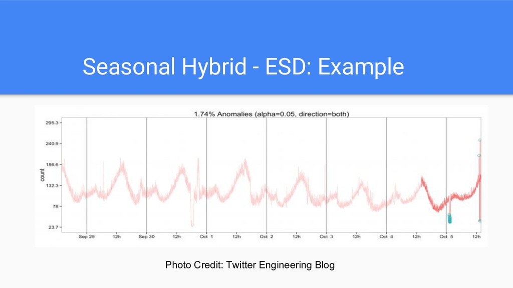
22. Seasonal Hybrid - ESD • Algorithm invented at Twitter in 2015. • Two components: ◦ Seasonal Decomposition: Remove seasonal patterns from the time series ◦ ESD: Iteratively test for outliers in the time series. • Remove periodic patterns from the time series, then identify anomalies with the remaining “core” of the time series.
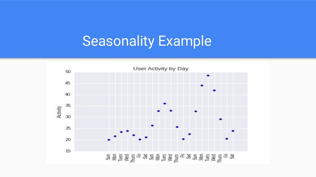
23. Seasonal Decomposition • Time Series Decomposition breaks a time series down into three components: a. Trend Component b. Seasonal Component c. Residual (or Random) Component • The trend component contains the “meat” of the time series that we are interested in. • The Seasonal component represents periodic patterns, and the Residual component reflects random noise.
24. Seasonality Example
25. Extreme Studentized Deviate • ESD is a statistical procedure to iteratively test for outliers in a dataset. • Specify the alpha level and the maximum number of anomalies to identify. • ESD naturally applies a statistical correction to compensate for multiple hypothesis testing.
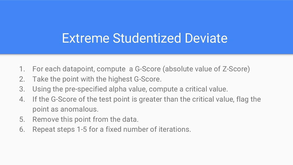
26. Extreme Studentized Deviate 1. For each datapoint, compute a G-Score (absolute value of Z-Score) 2. Take the point with the highest G-Score. 3. Using the pre-specified alpha value, compute a critical value. 4. If the G-Score of the test point is greater than the critical value, flag the point as anomalous. 5. Remove this point from the data. 6. Repeat steps 1-5 for a fixed number of iterations.
27. Seasonal Hybrid - ESD: Example Photo Credit: Twitter Engineering Blog
28. Robust PCA • Created in 2009 by Candes et al. • Regular PCA identifies a low-rank representation of the data using Singular Value Decomposition. • Robust PCA identifies a low-rank representation, outliers, and noise. • Used by Netflix in the Robust Anomaly Detection (RAD) package.
29. Robust PCA • Specify thresholds for the singular values and the error value. • Iterate through the data: ◦ Apply Singular Value Decomposition. ◦ Using thresholds, categorize the data into “normal”, “outlier”, “noise”. ◦ Repeat until all points are classified.
30. Robust PCA - Example Source: Netflix Techblog
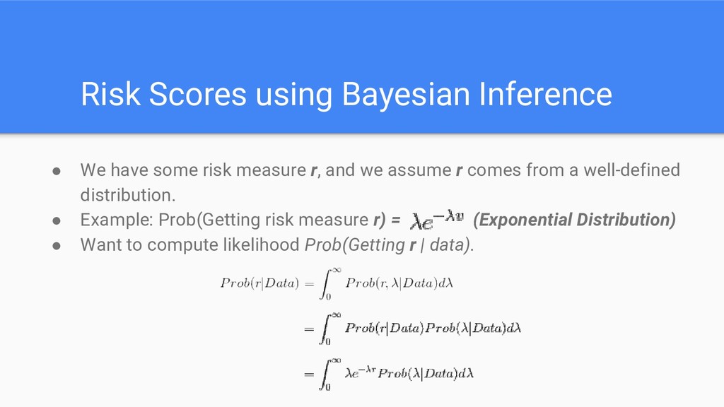
31. Risk Scores • When doing anomaly detection in practice, you want to treat it more as a regression problem rather than a classification problem. • Best practices recommend calculating the likelihood that a data point or event is anomalous and converting the likelihood into a risk score. • Risk scores should be from 0-100 because people more intuitively understand this scale.
32. Risk Scores using Bayesian Inference • We have some risk measure r, and we assume r comes from a well-defined distribution. • Example: Prob(Getting risk measure r) = (Exponential Distribution) • Want to compute likelihood Prob(Getting r | data).
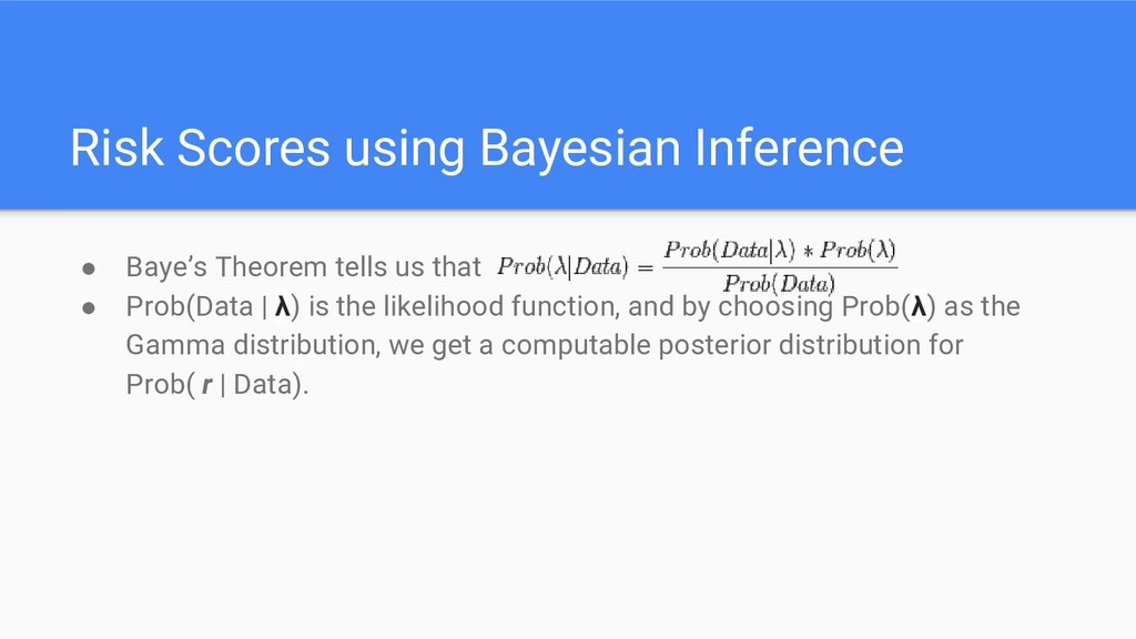
33. Risk Scores using Bayesian Inference • Baye’s Theorem tells us that • Prob(Data | λ) is the likelihood function, and by choosing Prob(λ) as the Gamma distribution, we get a computable posterior distribution for Prob( r | Data).
34. Risk Scores using Bayesian Inference
35. Testing your algorithms • Be sure to test algorithms in different environments. Just because it performs well in one environment does not mean it will generalize well to other environments. • Since anomalies are rare, create synthetic datasets with built-in anomalies. If you can’t identify the built-in anomalies, then you have a problem. • You should be constantly testing and fine-tuning your algorithms, so I recommend building a test harness to automate testing.
36. Questions?