Parametrized inversion framework for proppant volume in a hydraulically fractured reservoir

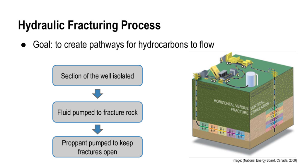
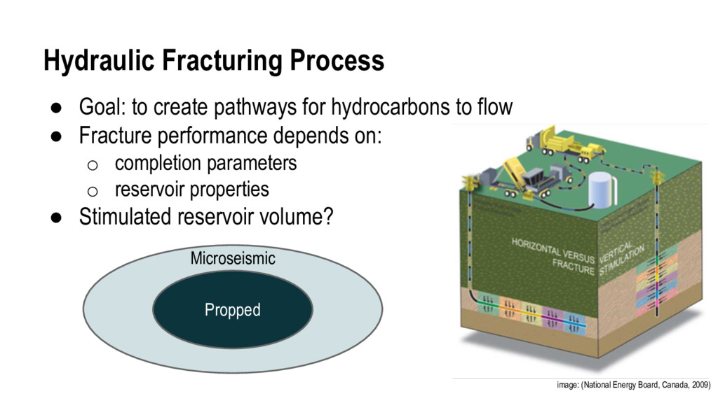
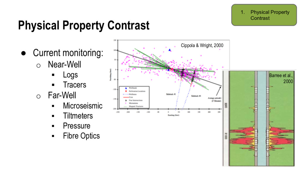
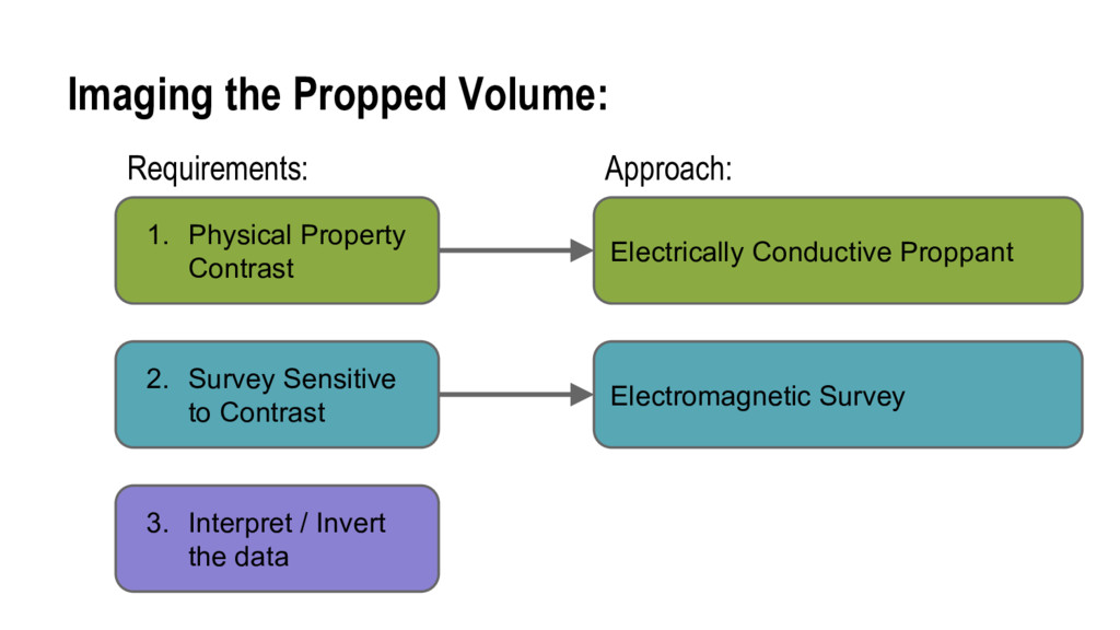
Hydraulic fracturing is an important technique to allow mobi- lization of hydrocarbons in tight reservoirs. Sand or ceramic proppant is pumped into the fractured reservoir to ensure frac- tures remain open and permeable after the hydraulic treatment. As such, the distribution of proppant is a controlling factor on where the reservoir is permeable and can be effectively drained. Methods to monitor the fracturing process, such as tiltmeters or microseismic, are not sensitive to proppant distri- butions in the subsurface after the fracturing treatment is com- plete (Cipolla and Wright, 2000).
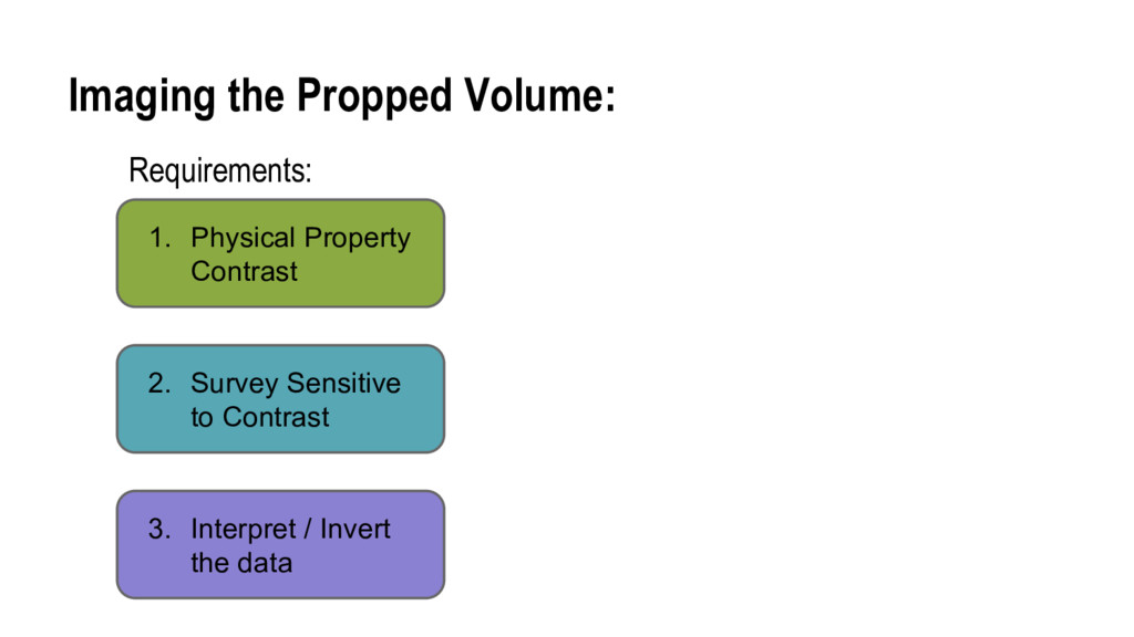
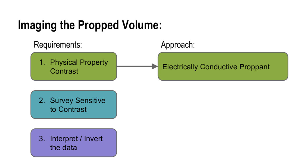
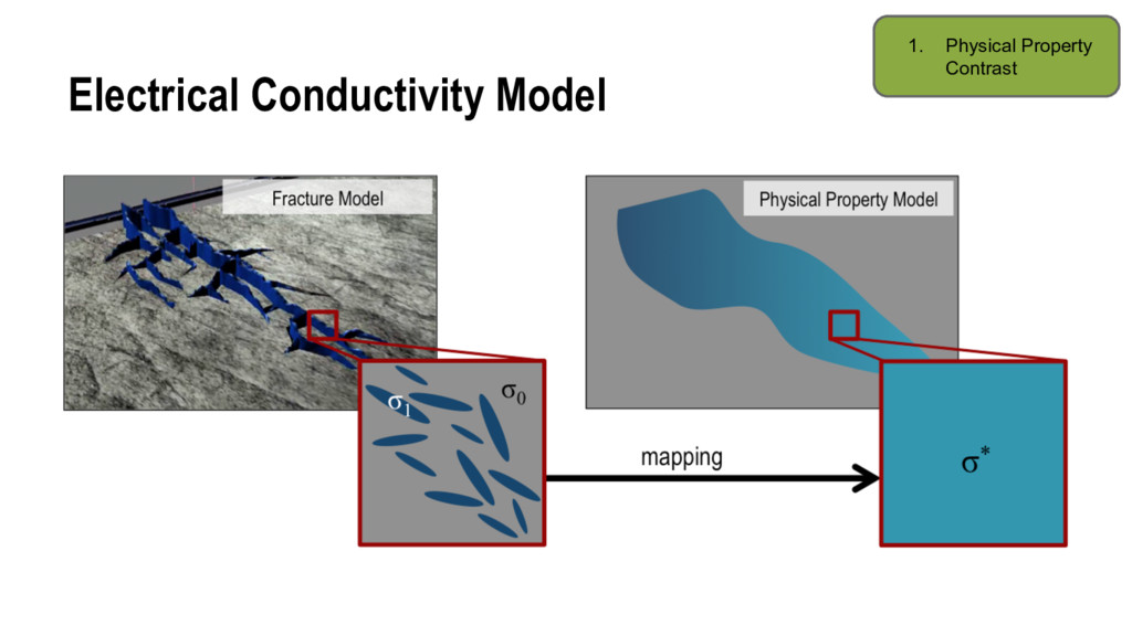
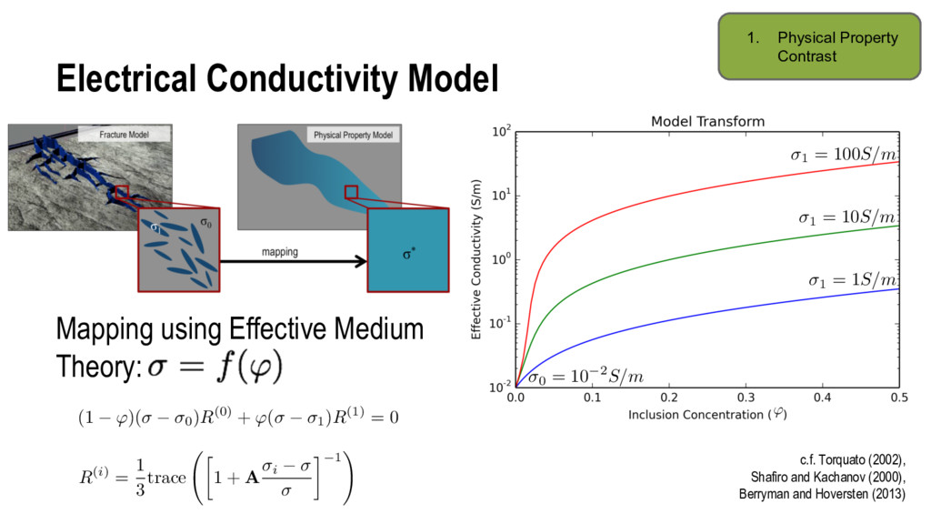
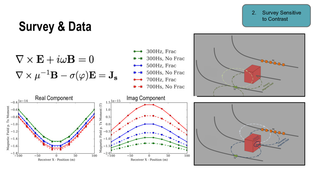
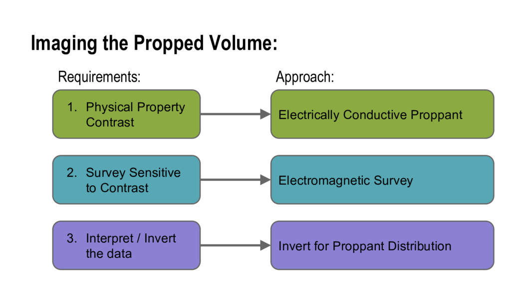
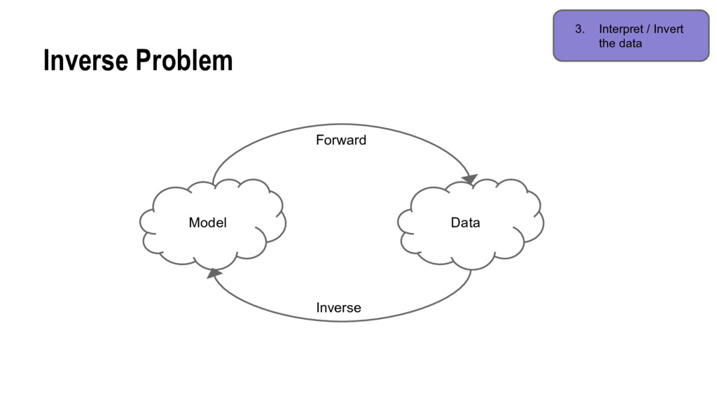
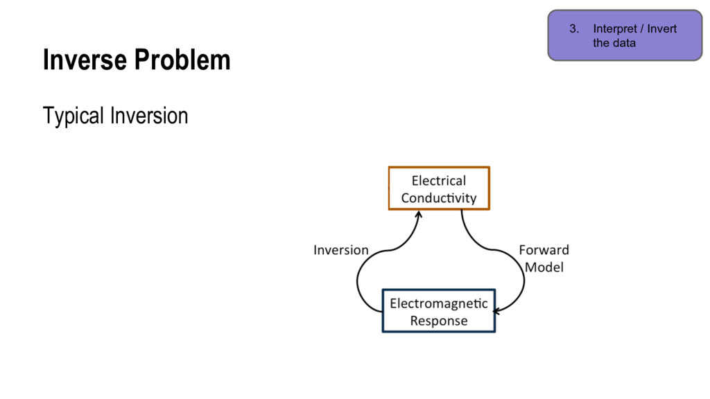
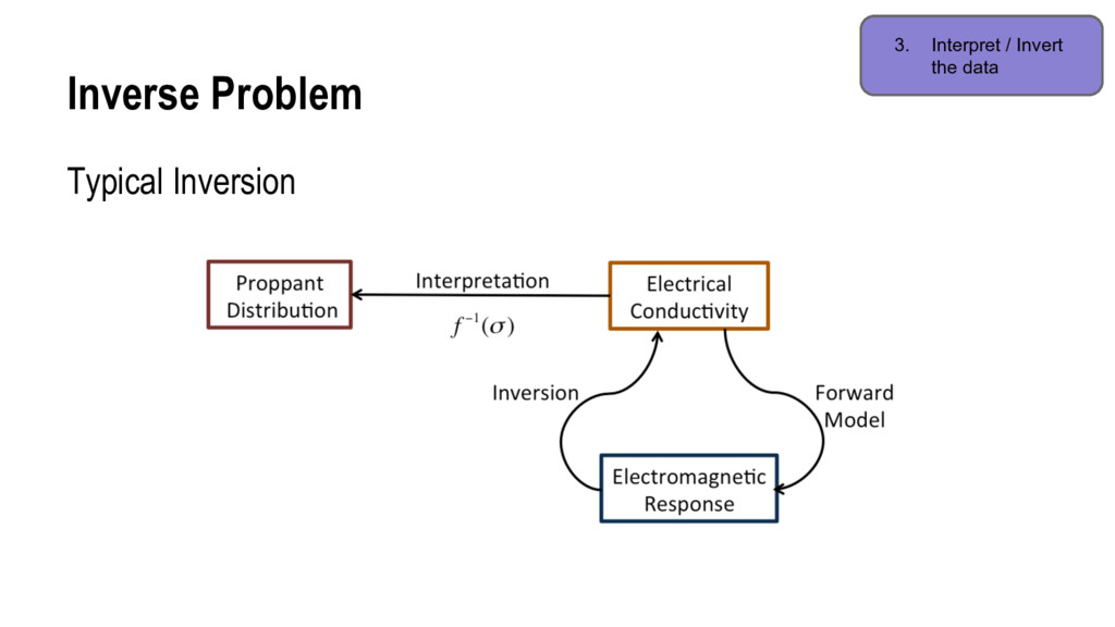
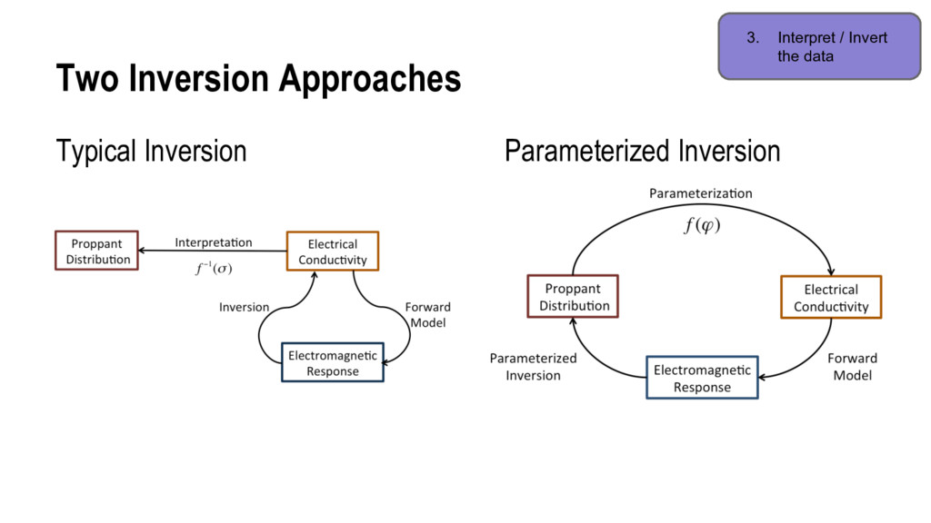
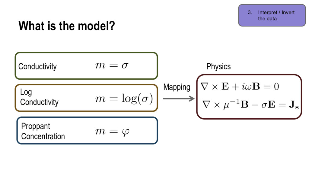
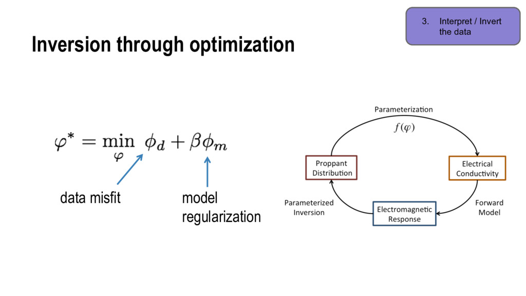
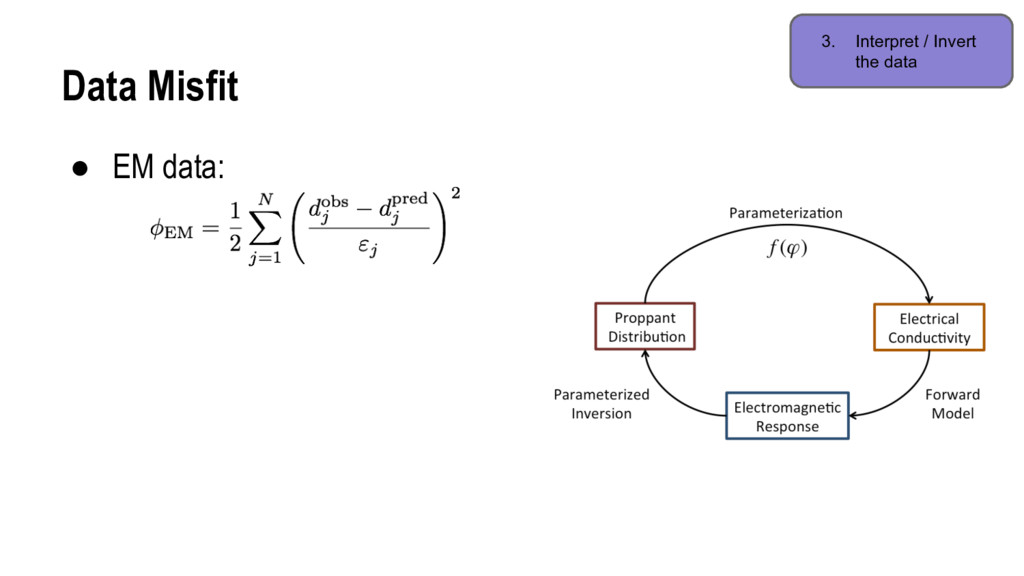
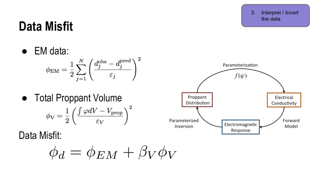
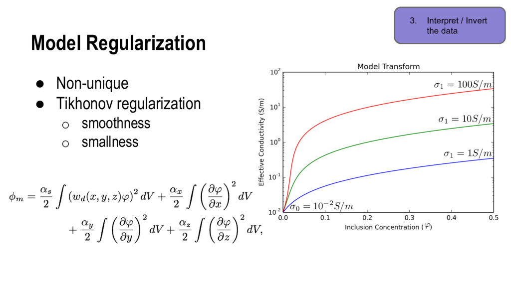
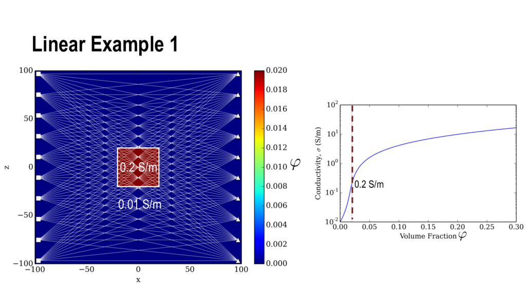
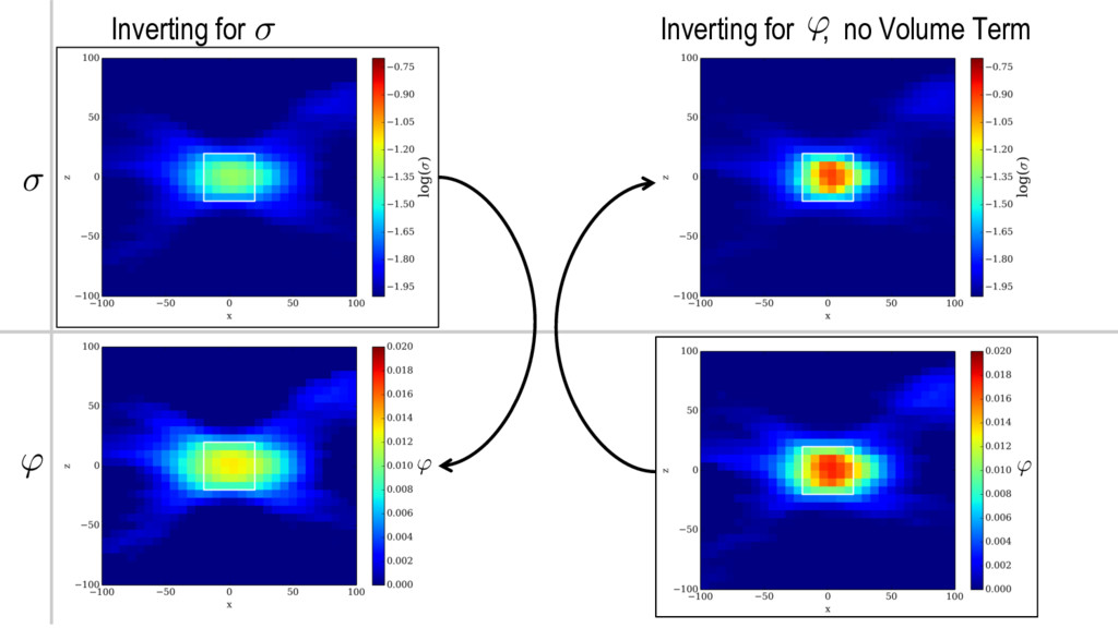
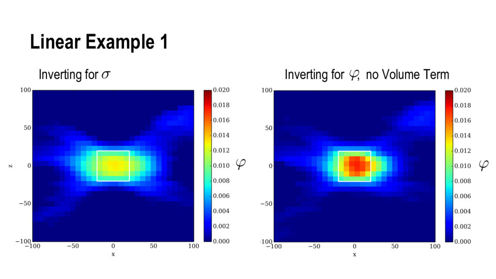
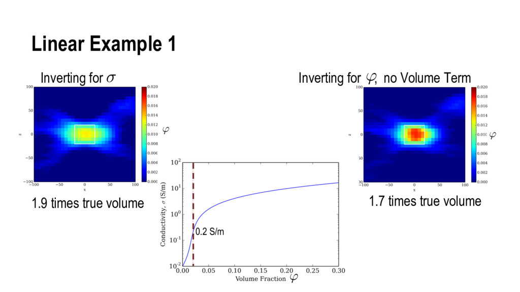
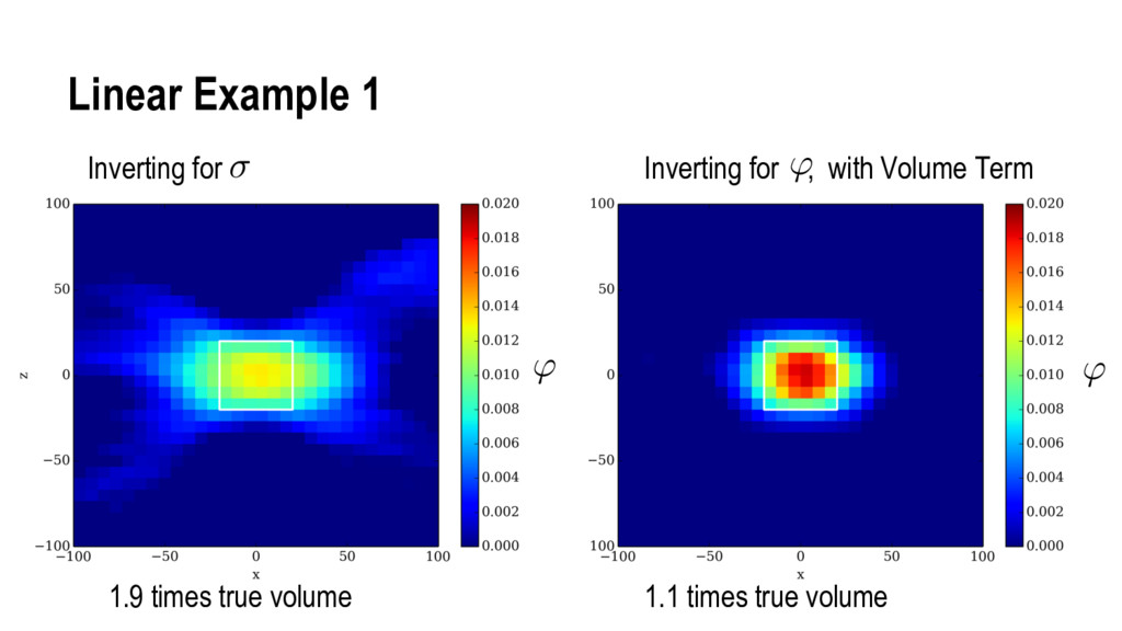
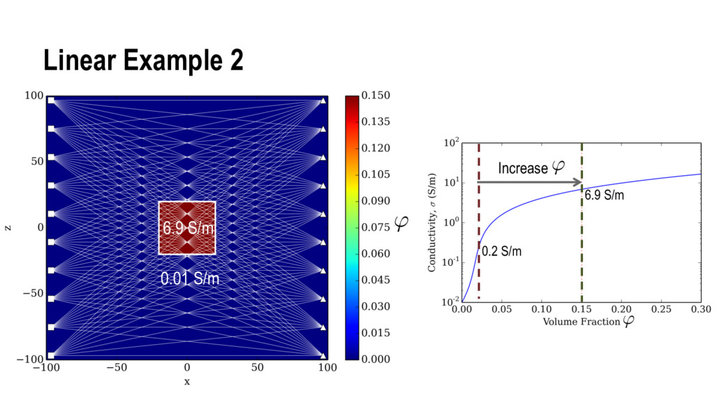
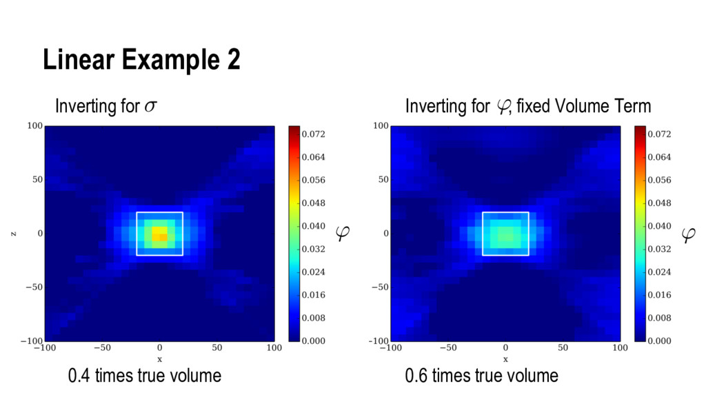
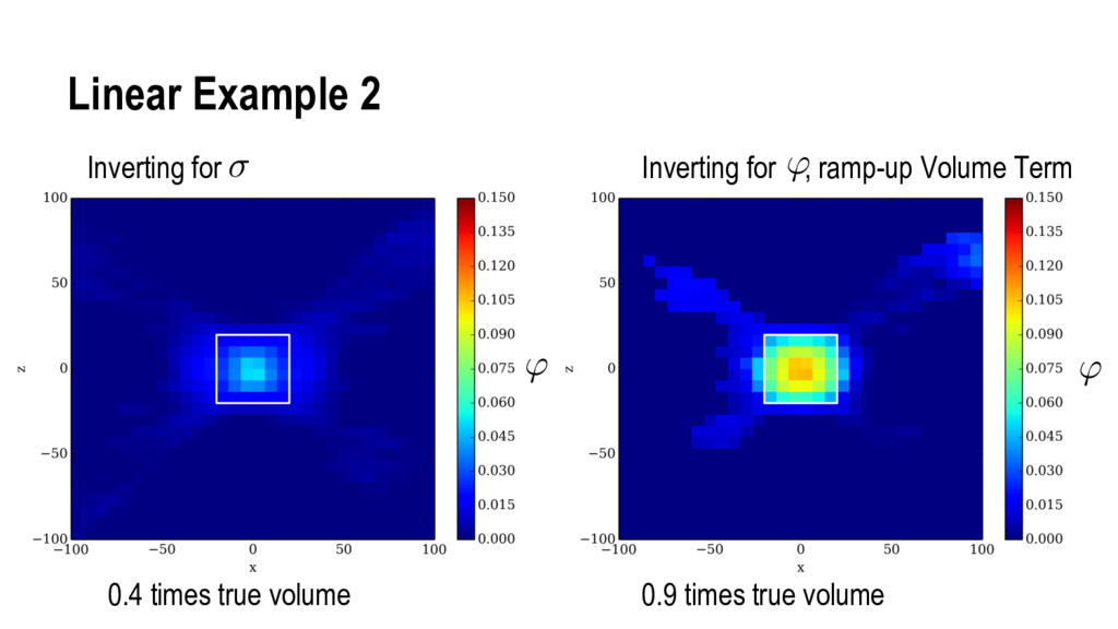
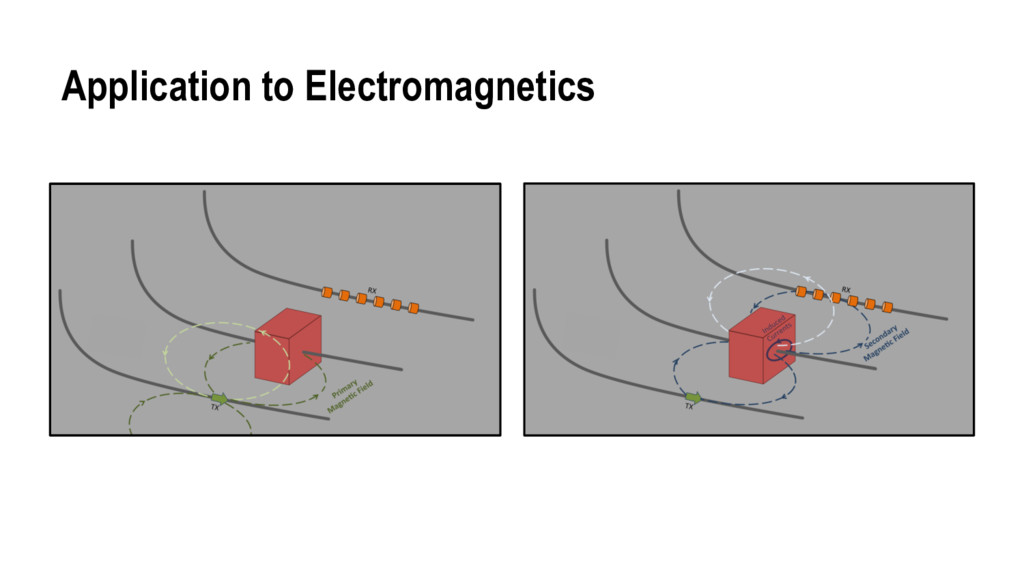
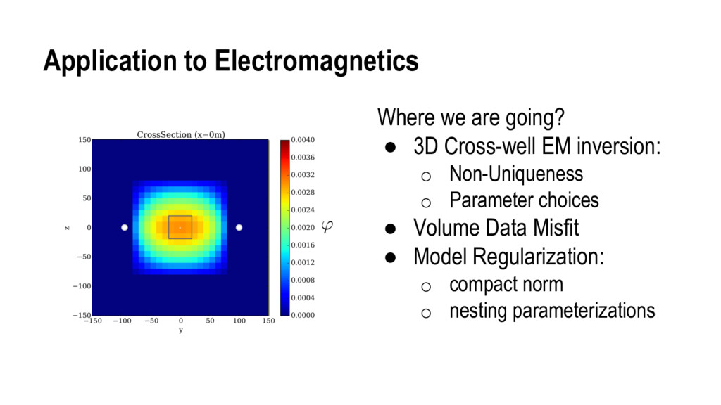
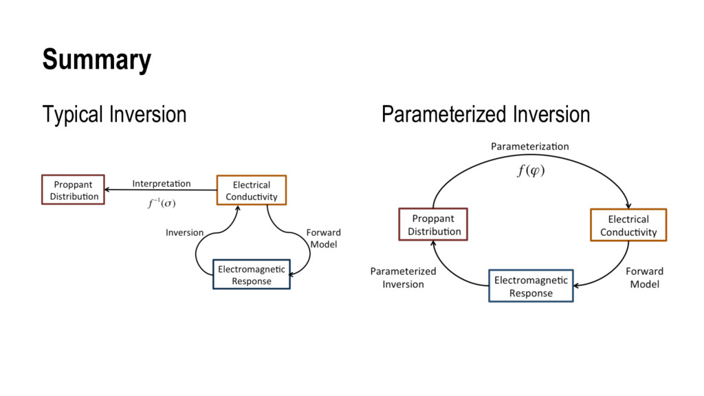
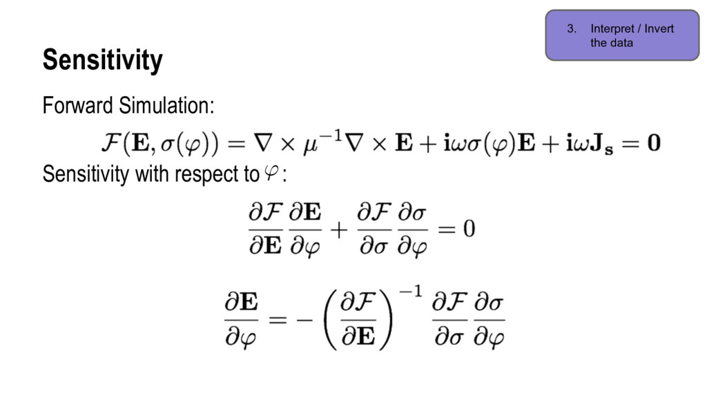
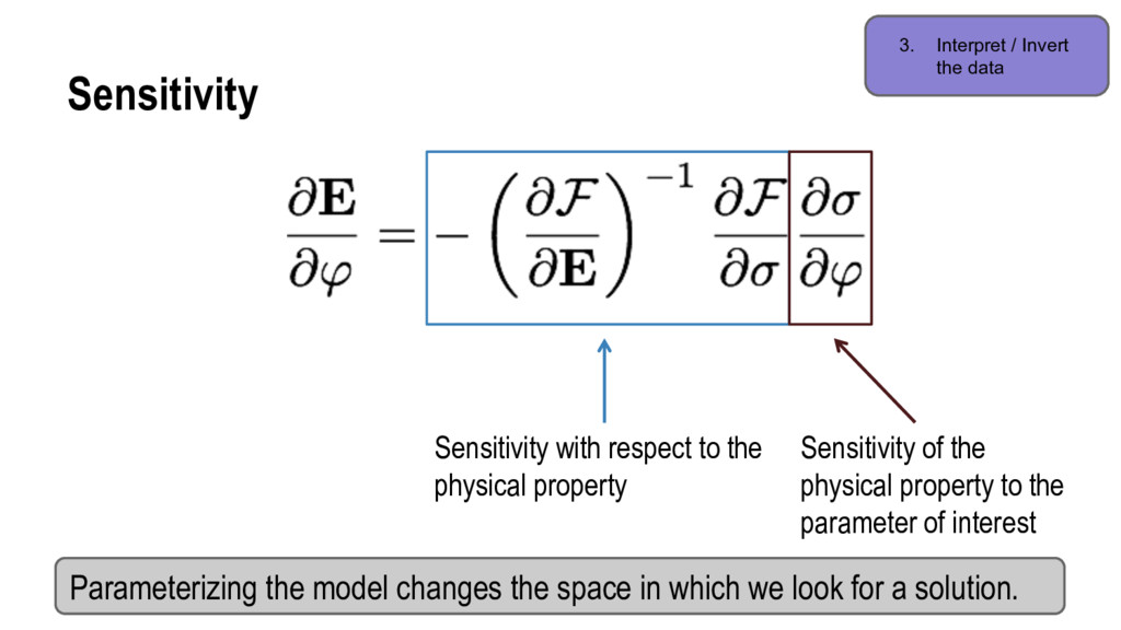
An electrically conductive proppant could create a signifi- cant physical property contrast between the propped region of the reservoir and the host rock. Electromagnetic geophysical methods can be used to image this property (Heagy and Olden- burg, 2013). However, traditional geophysical inversions are poorly constrained, requiring a-priori information to be in- corporated through known electrical properties. We examine a strategy to invert directly for the proppant volume using a parametrization of electrical conductivity in terms of proppant distribution within the reservoir.

Extended abstract available at: http://library.seg.org/doi/abs/10.1190/segam2014-1639.1

Transcript

1. SEG Denver October 28, 2014 Parameterized inversion framework for proppant volume in a hydraulically fractured reservoir Lindsey J. Heagy, Rowan Cockett & Douglas W. Oldenburg, UBC Geophysical Inversion Facility, University of British Columbia
2. • Goal: to create pathways for hydrocarbons to flow Hydraulic Fracturing Process image: (National Energy Board, Canada, 2009) Section of the well isolated Fluid pumped to fracture rock Proppant pumped to keep fractures open
3. • Goal: to create pathways for hydrocarbons to flow • Fracture performance depends on: o completion parameters o reservoir properties • Stimulated reservoir volume? Hydraulic Fracturing Process image: (National Energy Board, Canada, 2009) Propped Microseismic
4. Imaging the Propped Volume: 1. Physical Property Contrast 2. Survey Sensitive to Contrast 3. Interpret / Invert the data Requirements:
5. Physical Property Contrast • Current monitoring: o Near-Well § Logs § Tracers o Far-Well § Microseismic § Tiltmeters § Pressure § Fibre Optics 1. Physical Property Contrast Cippola & Wright, 2000 Barree et al., 2000
6. Imaging the Propped Volume: 1. Physical Property Contrast Electrically Conductive Proppant 2. Survey Sensitive to Contrast 3. Interpret / Invert the data Requirements: Approach:
7. Electrical Conductivity Model - SC EMT (note that other models, empirical, analytical or numerical possible) - also need to bring in that we are assuming that we know the background conductivity model 1. Physical Property Contrast
8. Electrical Conductivity Model 1. Physical Property Contrast c.f. Torquato (2002), Shafiro and Kachanov (2000), Berryman and Hoversten (2013) R(i) = 1 3 trace  1 + A i 1 ! (1 ')( 0)R(0) + '( 1)R(1) = 0 Mapping using Effective Medium Theory: 0 = 10 2S/m 1 = 1S/m 1 = 10S/m 1 = 100S/m '
9. Imaging the Propped Volume: 1. Physical Property Contrast Electrically Conductive Proppant 2. Survey Sensitive to Contrast Electromagnetic Survey 3. Interpret / Invert the data Requirements: Approach:
10. Survey & Data 2. Survey Sensitive to Contrast Real Component Imag Component
11. Imaging the Propped Volume: 1. Physical Property Contrast Electrically Conductive Proppant 2. Survey Sensitive to Contrast Electromagnetic Survey 3. Interpret / Invert the data Invert for Proppant Distribution Requirements: Approach:
12. Inverse Problem 3. Interpret / Invert the data Model Data Forward Inverse
13. Inverse Problem Typical Inversion 3. Interpret / Invert the data
14. Inverse Problem Typical Inversion 3. Interpret / Invert the data
15. Two Inversion Approaches Typical Inversion 3. Interpret / Invert the data Parameterized Inversion
16. What is the model? 3. Interpret / Invert the data Conductivity Log Conductivity Proppant Concentration m = m = log( ) m = ' Mapping r ⇥ µ 1B E = Js r ⇥ E + i!B = 0 Physics
17. Inversion through optimization 3. Interpret / Invert the data data misfit model regularization
18. Data Misfit • EM data: 3. Interpret / Invert the data
19. Data Misfit • EM data: • Total Proppant Volume Data Misfit: 3. Interpret / Invert the data d = EM + V V
20. Model Regularization • Non-unique • Tikhonov regularization o smoothness o smallness 3. Interpret / Invert the data 0 = 10 2S/m 1 = 1S/m 1 = 10S/m 1 = 100S/m '
21. (does it work?)
22. Linear Example 1 ' 0.2 S/m 0.01 S/m 0.2 S/m '
23. Inverting for , no Volume Term 1.9 times true volume Inverting for ' ' ' '
24. Linear Example 1 Inverting for , no Volume Term ' Inverting for ' '
25. Inverting for , no Volume Term ' ' Inverting for ' Linear Example 1 0.2 S/m ' 1.9 times true volume 1.7 times true volume
26. Linear Example 1 Inverting for , with Volume Term ' 1.9 times true volume 1.1 times true volume Inverting for ' '
27. Linear Example 2 ' 6.9 S/m 0.01 S/m 0.2 S/m ' Increase ' 6.9 S/m
28. Linear Example 2 Inverting for , fixed Volume Term ' 0.4 times true volume 0.6 times true volume Inverting for ' '
29. Linear Example 2 Inverting for , ramp-up Volume Term ' 0.4 times true volume 0.9 times true volume Inverting for ' '
30. Application to Electromagnetics
31. Application to Electromagnetics Where we are going? • 3D Cross-well EM inversion: o Non-Uniqueness o Parameter choices • Volume Data Misfit • Model Regularization: o compact norm o nesting parameterizations '
32. Summary Typical Inversion Parameterized Inversion
33. Acknowledgements • Seogi Kang • SimPEG contributors • Mike Wilt, Jiuping Chen, Nestor Cuevas and Ping Zhang • UBC GIF • NSERC Thank you! SEG Denver October 28, 2014
34. References • Barree, R. D., Fisher, M. K. & Woodroof, R. a. A Practical Guide to Hydraulic Fracture Diagnostic Technologies. Pap. SPE 77442, Present. SPE Annu. Tech. Conf. Exhib. held San Antonio, Texas, 29 Sept. - 2 Oct. (2002). doi:10.2523/77442-MS • Berryman, J. G. & Hoversten, G. M. Modelling electrical conductivity for earth media with macroscopic fluid-filled fractures. Geophys. Prospect. 61, 471–493 (2013). • Bruggeman, D. A. G. The calculation of various physical constants of heterogeneous substances. I. The dielectric constants and conductivities of mixtures composed of isotropic substances. Ann. Phys. 416, 636–664 (1935). • Cipolla, C. L. & Wright, C. A. Diagnostic Techniques to Understand Hydraulic Fracturing: What? Why? and How? SPE 59735, Present. 2000 SPE/CERI Gas Technol. Symp. held Calgary, Alberta, Canada, 3-5 April (2000). • National Energy Board, Canada (2009) http://www.neb-one.gc.ca/clf- nsi/archives/rnrgynfmtn/nrgyrprt/ntrlgs/prmrndrstndngshlgs2009/prmrndrstndngshlgs2009-eng.html • Oldenburg, D. & Li, Y. Inversion for applied geophysics: A tutorial. Investig. Geophys. 1–85 (2005). at <http://www.eoas.ubc.ca/courses/eosc454/content/Papers/Case Histories/Inversion Tutorial Oldenburg and Li 2005.pdf> • Shafiro, B. & Kachanov, M. Anisotropic effective conductivity of materials with nonrandomly oriented inclusions of diverse ellipsoidal shapes. J. Appl. Phys. 87, 8561–8569 (2000). • Torquato, S. Random Heterogeneous Materials: Microstructure and Macroscopic Properties. (Springer, 2002).
35. Sensitivity Forward Simulation: Sensitivity with respect to : 3. Interpret / Invert the data '
36. Sensitivity 3. Interpret / Invert the data Sensitivity with respect to the physical property Sensitivity of the physical property to the parameter of interest Parameterizing the model changes the space in which we look for a solution.