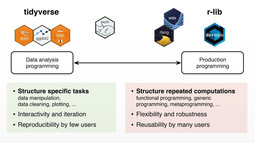
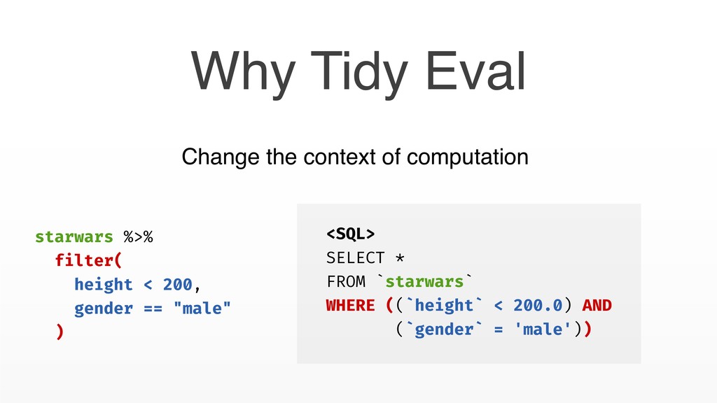
manipulation, data cleaning, plotting, ... • Interactivity and iteration • Reproducibility by few users • Structure repeated computations functional programming, generic programming, metaprogramming, ... • Flexibility and robustness • Reusability by many users r-lib tidyverse
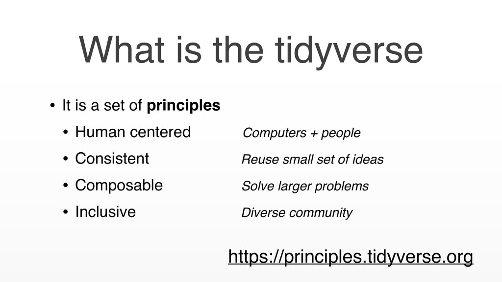
principles • Human centered Computers + people • Consistent Reuse small set of ideas • Composable Solve larger problems • Inclusive Diverse community https://principles.tidyverse.org
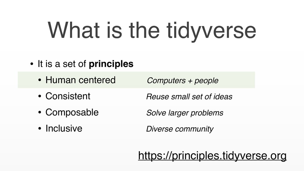
principles • Human centered Computers + people • Consistent Reuse small set of ideas • Composable Solve larger problems • Inclusive Diverse community https://principles.tidyverse.org
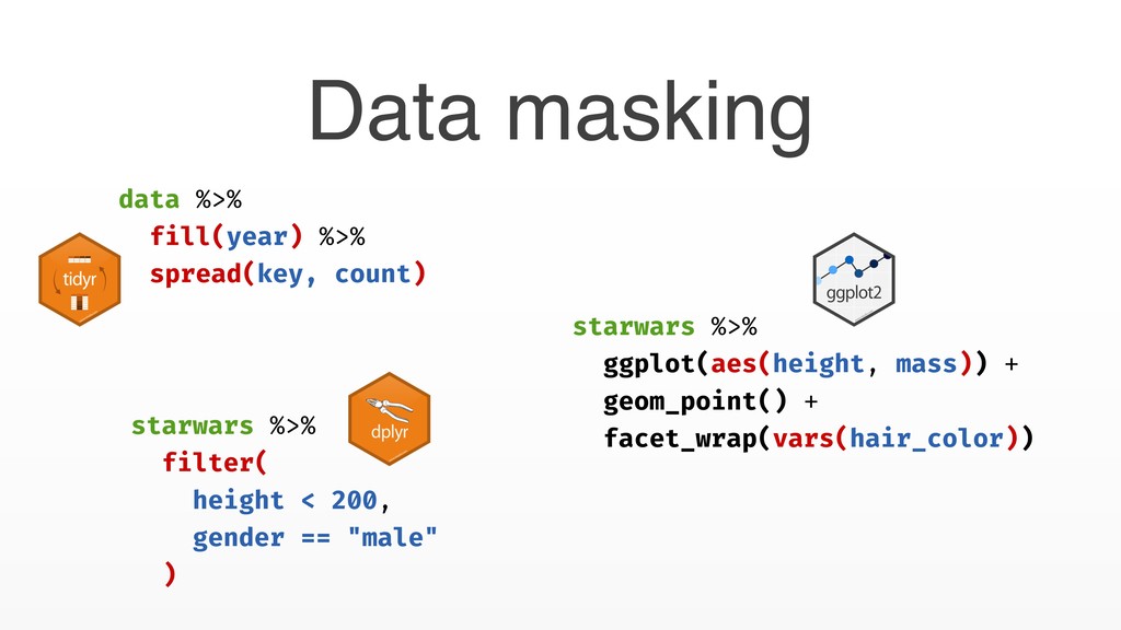
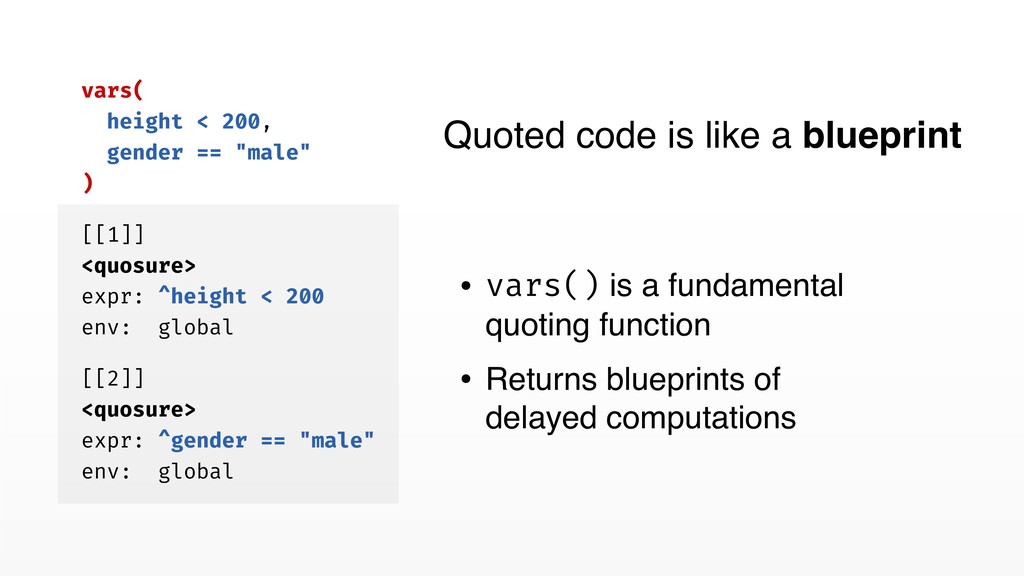
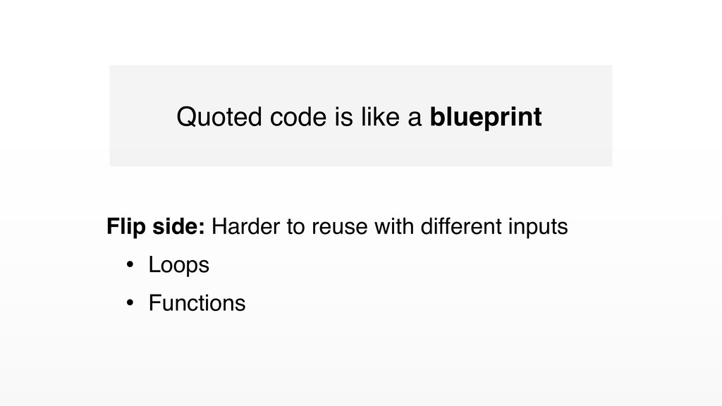
gender == "male" ) [[1]] <quosure> expr: ^height < 200 env: global [[2]] <quosure> expr: ^gender == "male" env: global • vars() is a fundamental quoting function • Returns blueprints of delayed computations
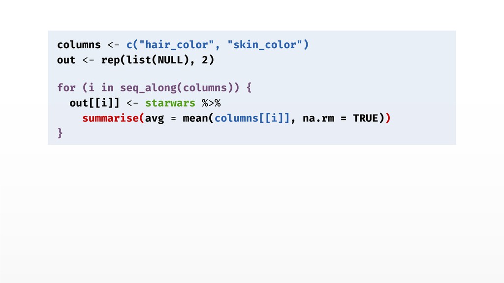
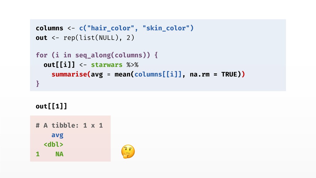
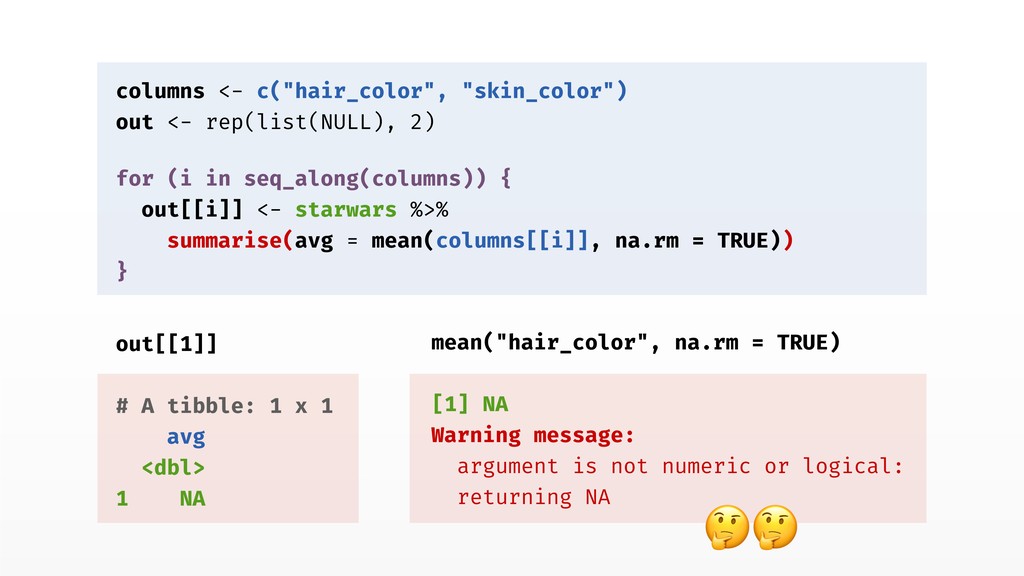
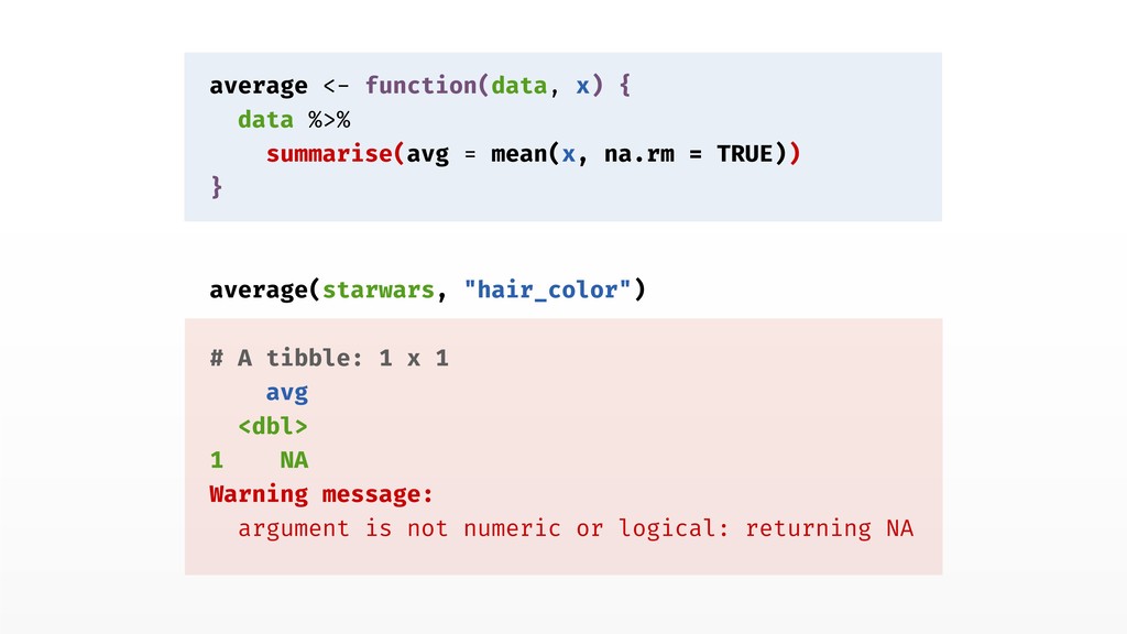
in seq_along(columns)) { out[[i]] <- starwars %>% summarise(avg = mean(columns[[i]], na.rm = TRUE)) } out[[1]] # A tibble: 1 x 1 avg <dbl> 1 NA mean("hair_color", na.rm = TRUE) [1] NA Warning message: argument is not numeric or logical: returning NA
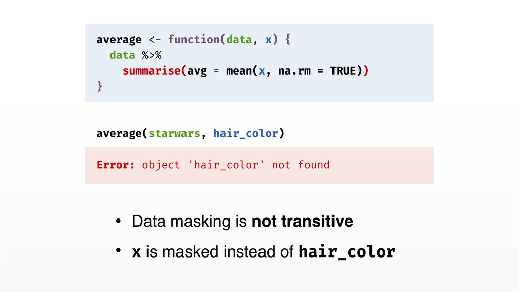
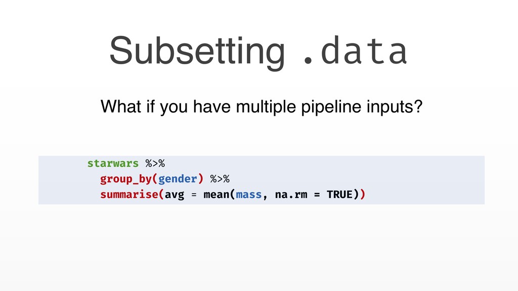
na.rm = TRUE)) } average(starwars, hair_color) Error: object 'hair_color' not found • Data masking is not transitive • x is masked instead of hair_color
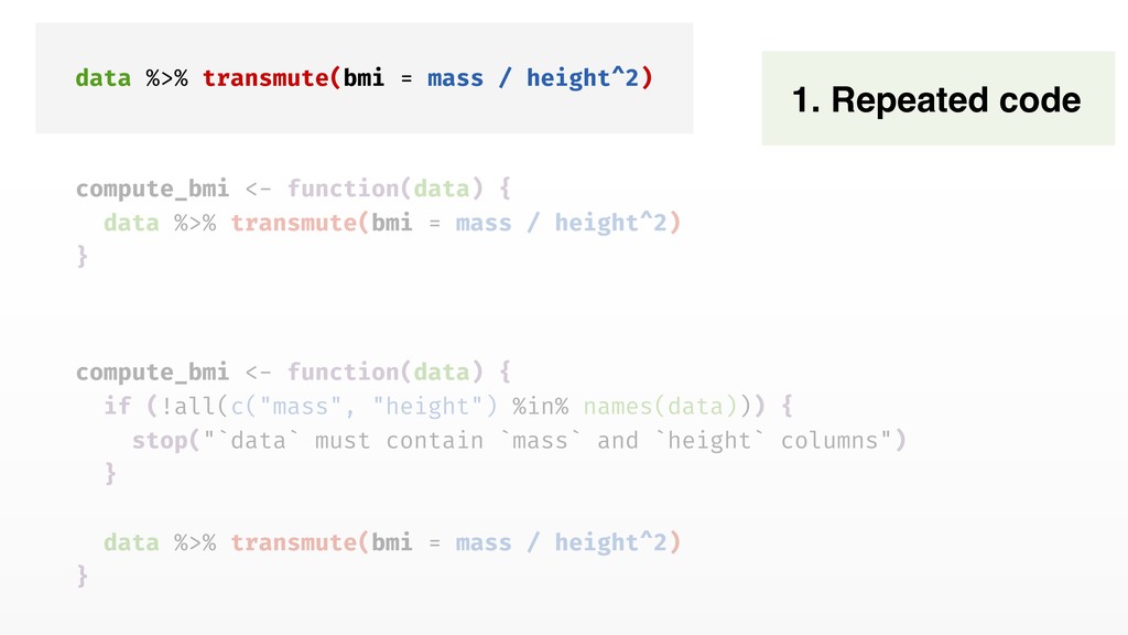
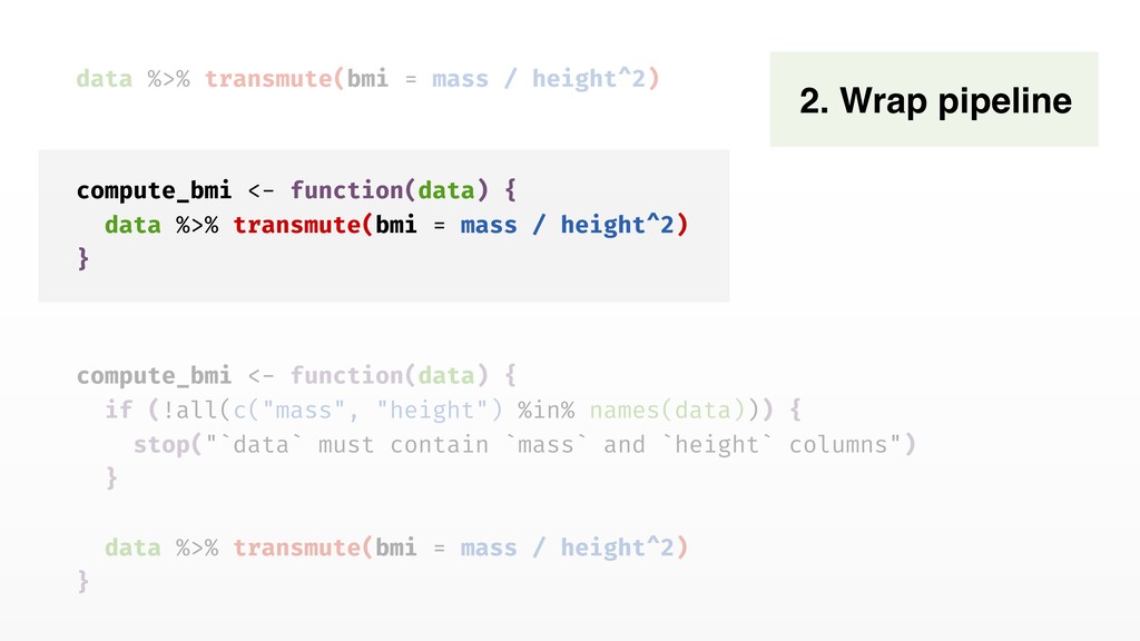
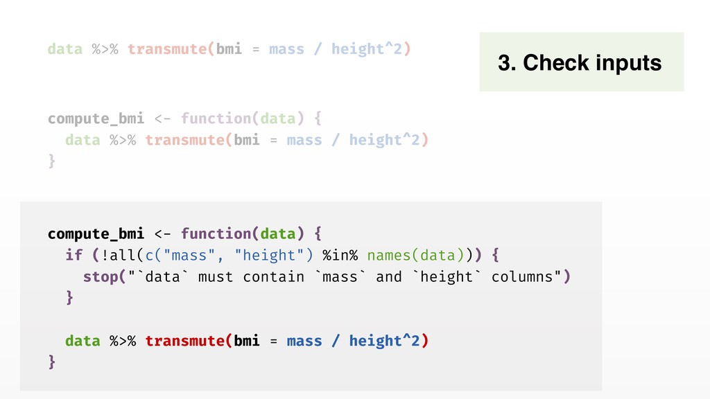
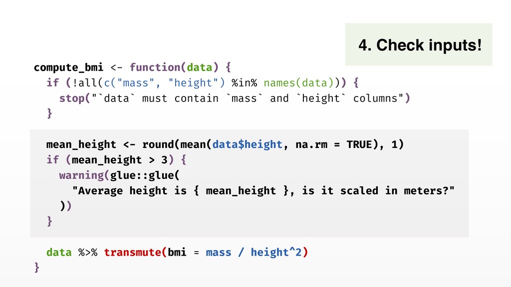
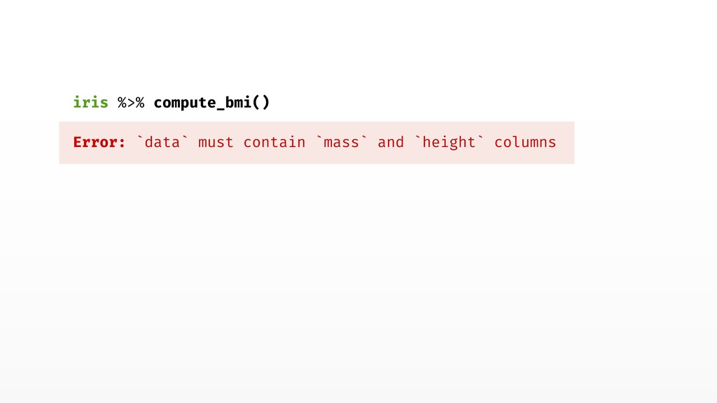
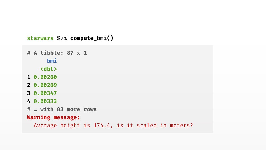
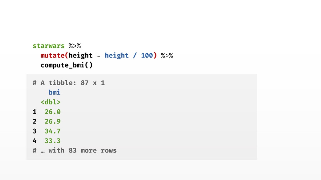
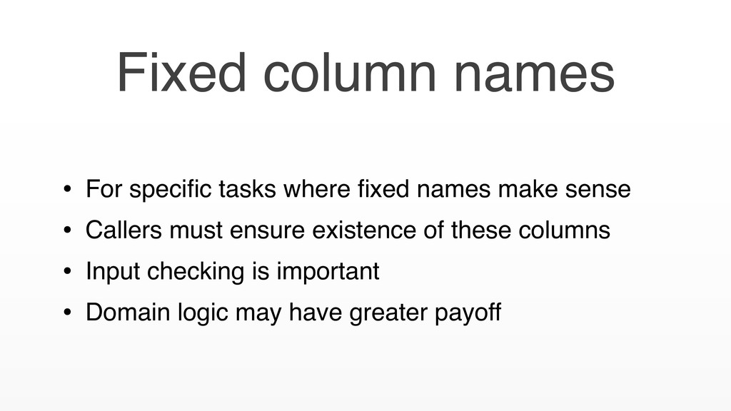
stop("`data` must contain `mass` and `height` columns") } mean_height <- round(mean(data$height, na.rm = TRUE), 1) if (mean_height > 3) { warning(glue::glue( "Average height is { mean_height }, is it scaled in meters?" )) } data %>% transmute(bmi = mass / height^2) } 4. Check inputs!
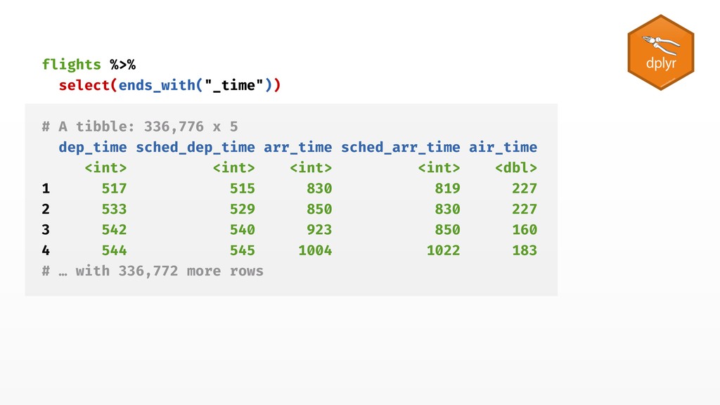
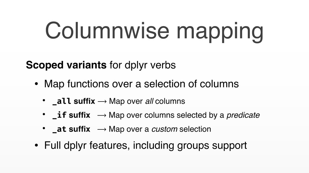
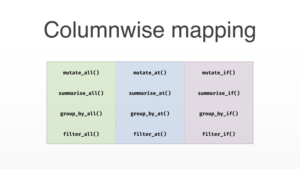
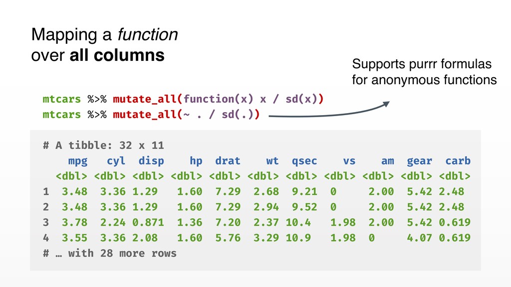
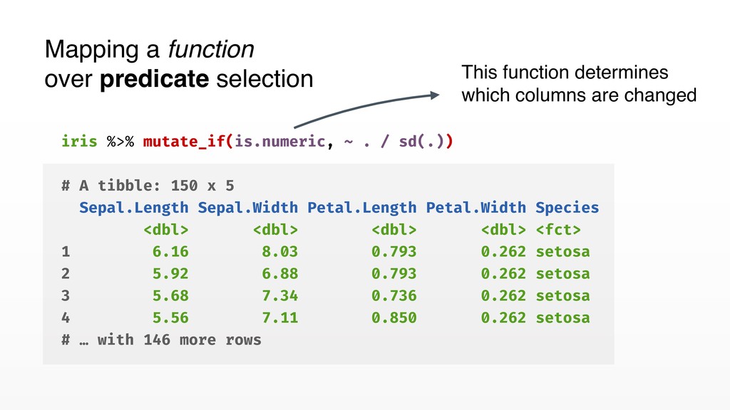
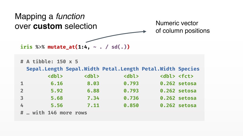
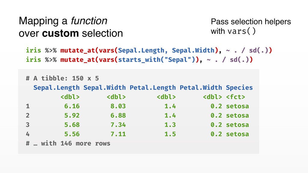
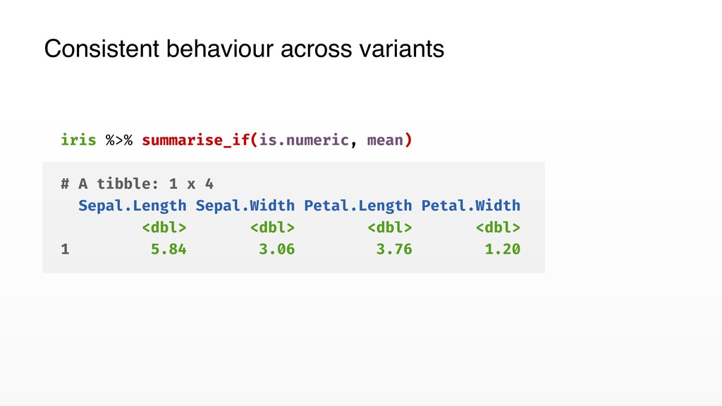
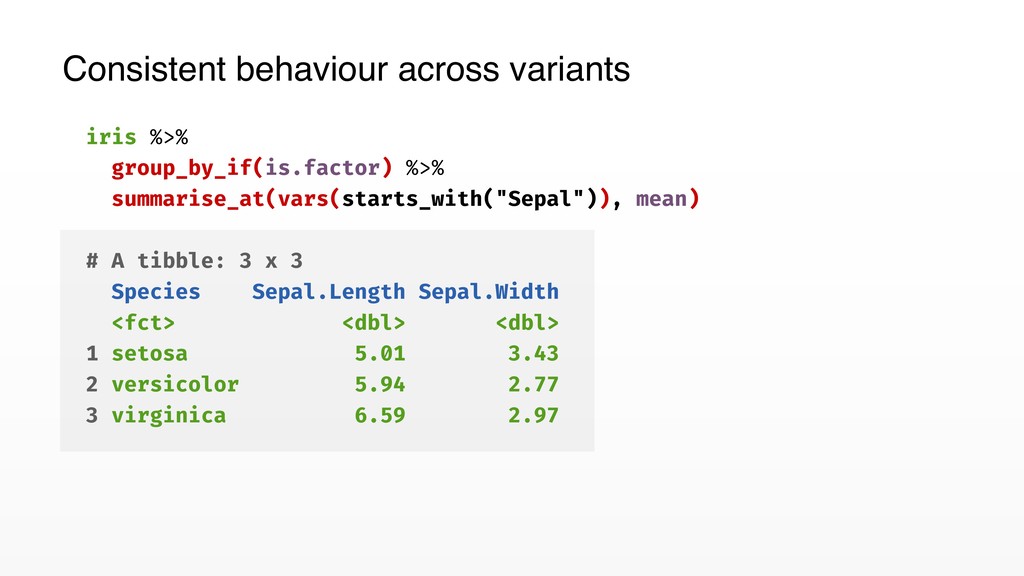
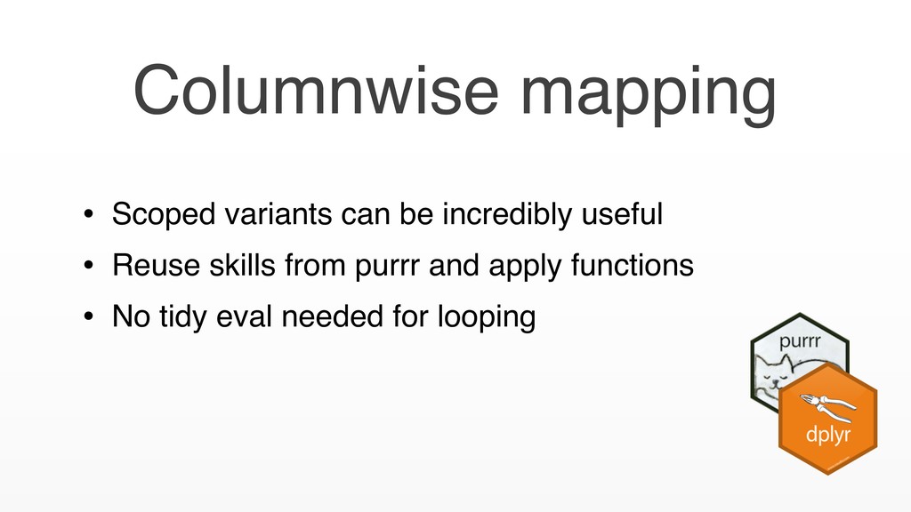
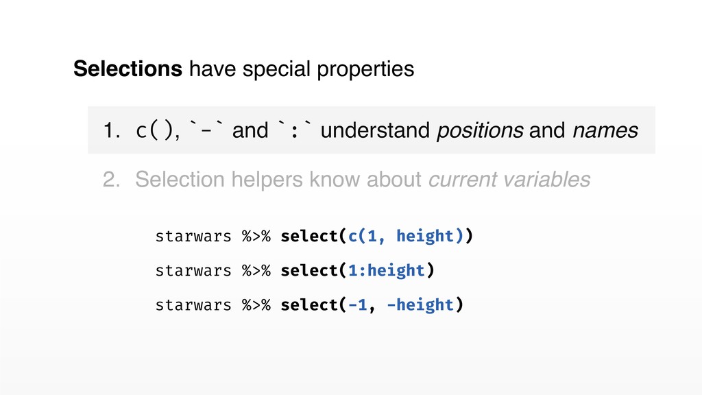
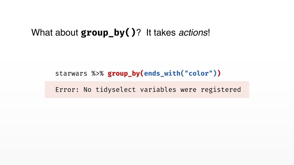
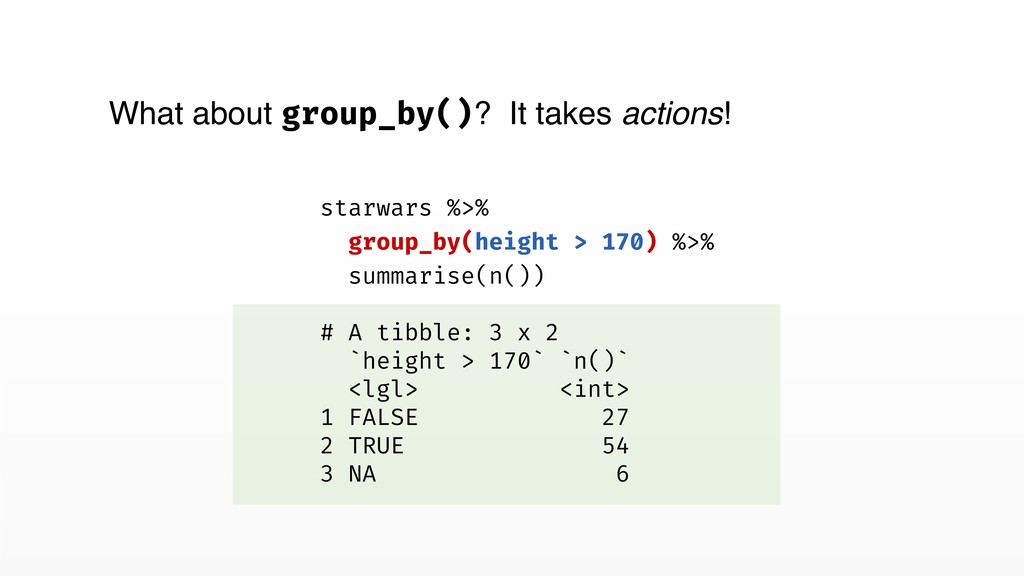
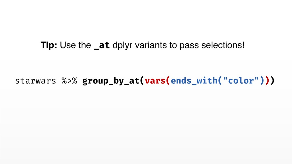
selection of columns • _all suffix ⟶ Map over all columns • _if suffix ⟶ Map over columns selected by a predicate • _at suffix ⟶ Map over a custom selection • Full dplyr features, including groups support Columnwise mapping
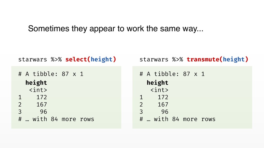
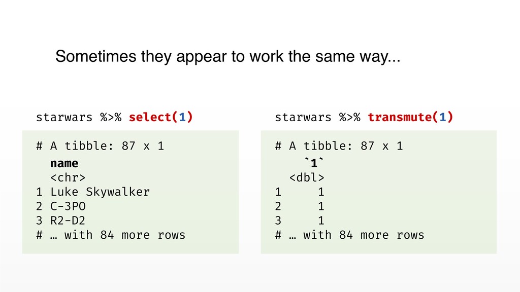
<chr> 1 Luke Skywalker 2 C-3PO 3 R2-D2 # … with 84 more rows starwars %>% transmute(1) # A tibble: 87 x 1 `1` <dbl> 1 1 2 1 3 1 # … with 84 more rows Sometimes they appear to work the same way...
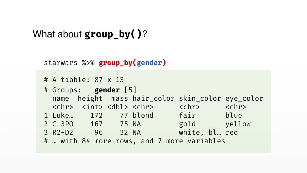
x 13 # Groups: gender [5] name height mass hair_color skin_color eye_color <chr> <int> <dbl> <chr> <chr> <chr> 1 Luke… 172 77 blond fair blue 2 C-3PO 167 75 NA gold yellow 3 R2-D2 96 32 NA white, bl… red # … with 84 more rows, and 7 more variables
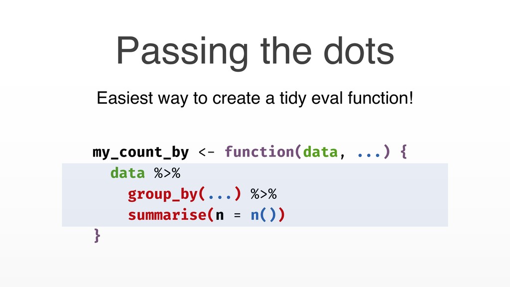
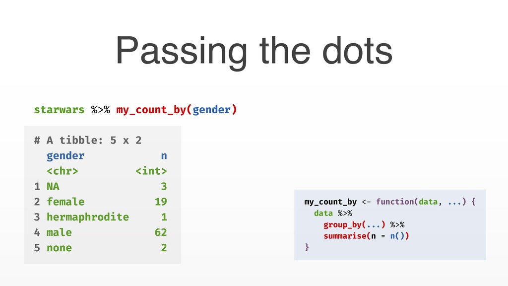
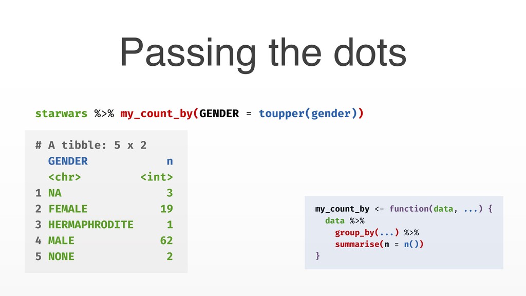
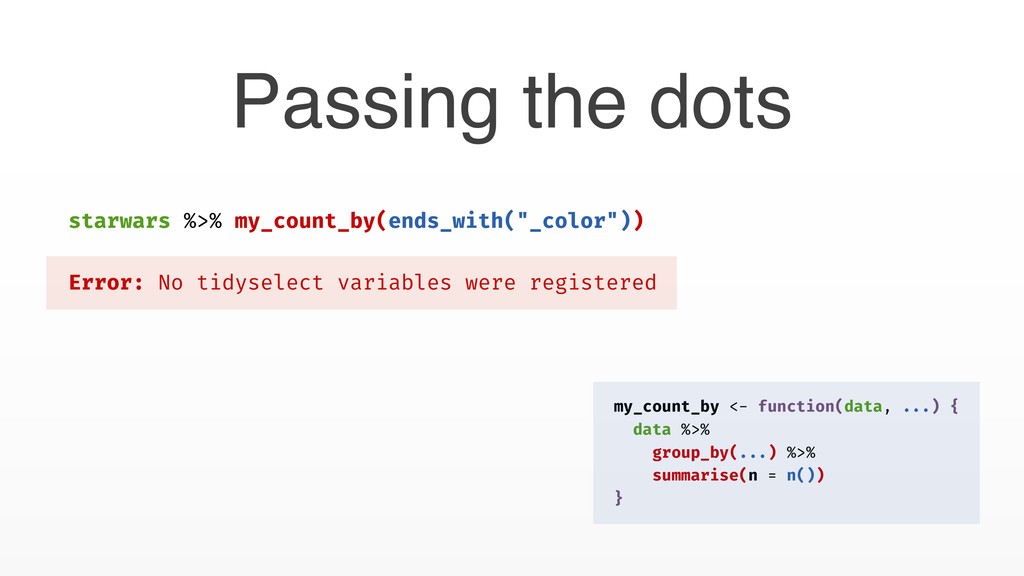
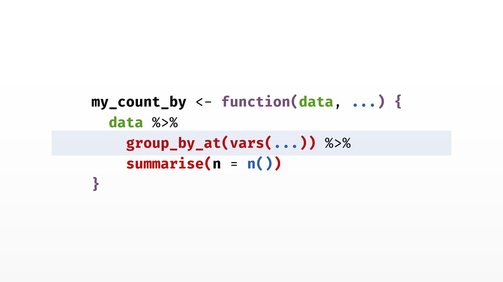
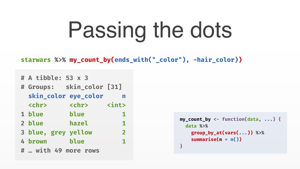
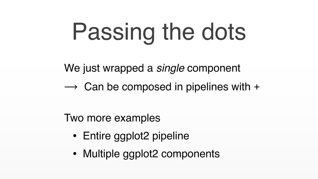
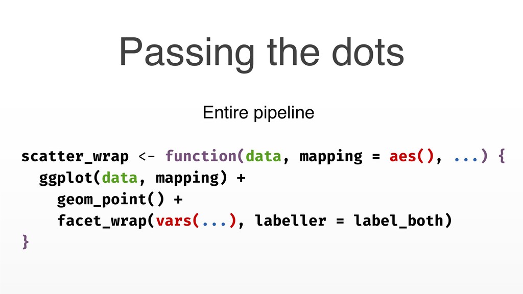
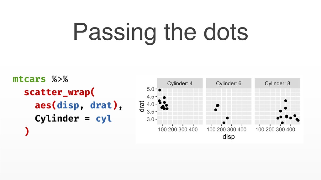
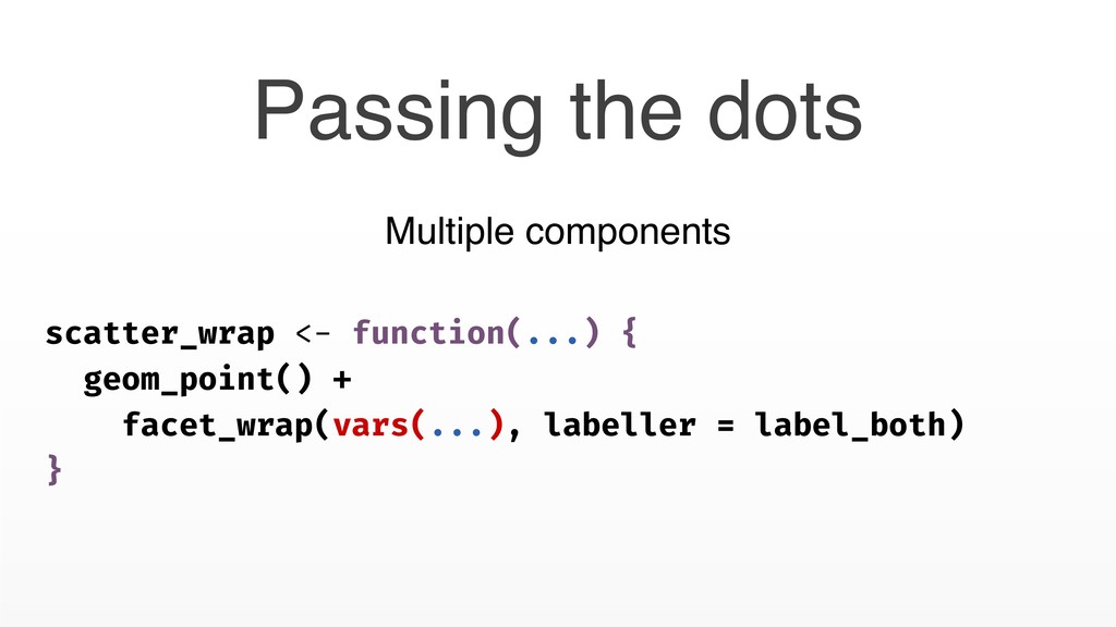
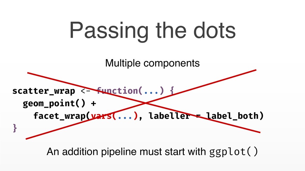
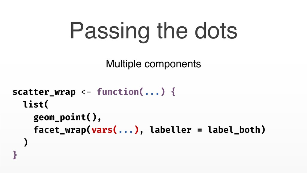
# Groups: skin_color [31] skin_color eye_color n <chr> <chr> <int> 1 blue blue 1 2 blue hazel 1 3 blue, grey yellow 2 4 brown blue 1 # … with 49 more rows my_count_by <- function(data, ...) { data %>% group_by_at(vars(...)) %>% summarise(n = n()) } Passing the dots
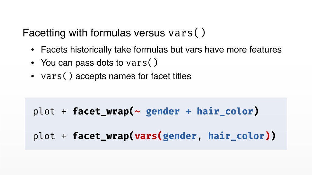
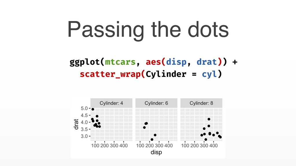
Facetting with formulas versus vars() • Facets historically take formulas but vars have more features • You can pass dots to vars() • vars() accepts names for facet titles
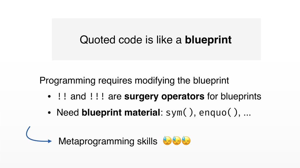
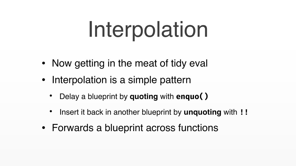
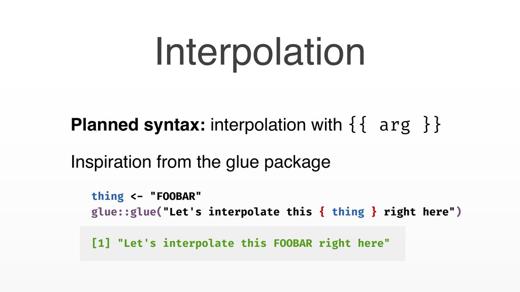
Interpolation is a simple pattern • Delay a blueprint by quoting with enquo() • Insert it back in another blueprint by unquoting with !! • Forwards a blueprint across functions Interpolation
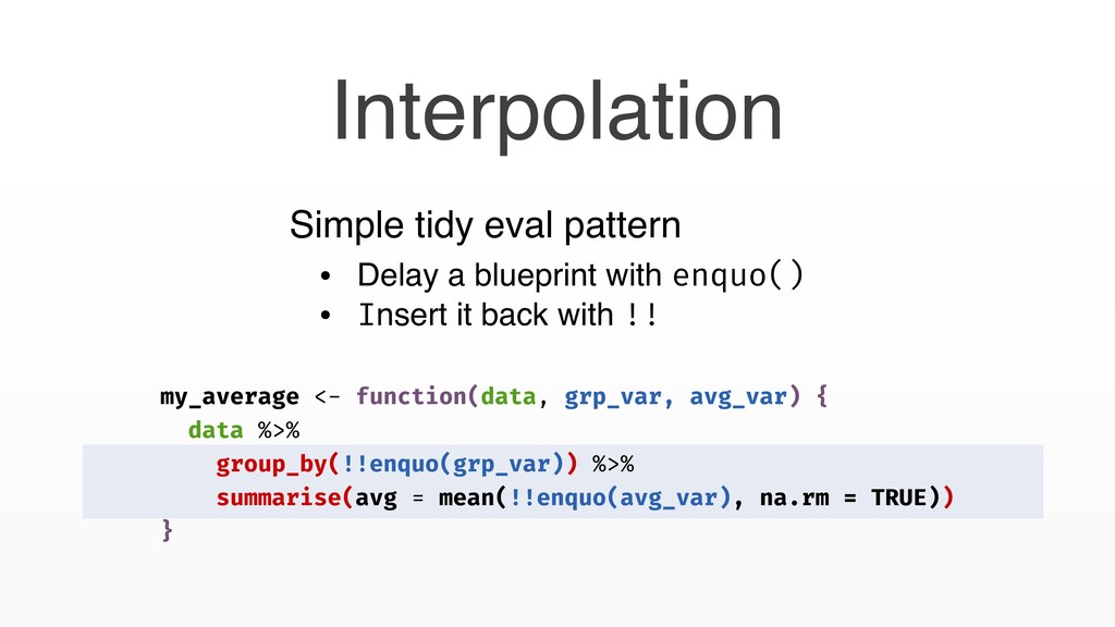
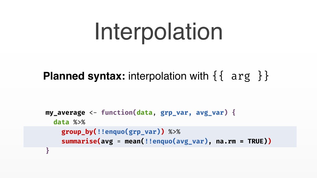
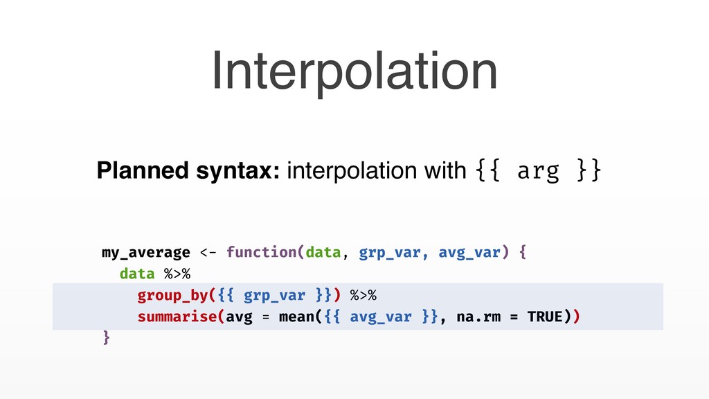
summarise(avg = mean(!!enquo(avg_var), na.rm = TRUE)) } Simple tidy eval pattern • Delay a blueprint with enquo() • Insert it back with !! Interpolation
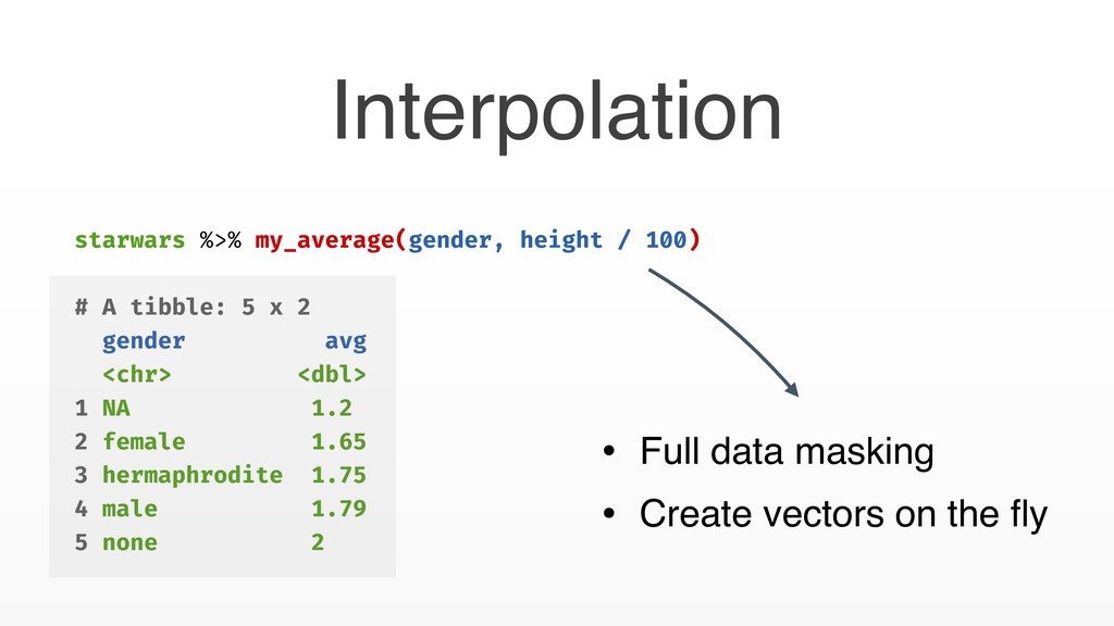
x 2 gender avg <chr> <dbl> 1 NA 1.2 2 female 1.65 3 hermaphrodite 1.75 4 male 1.79 5 none 2 • Full data masking • Create vectors on the fly Interpolation
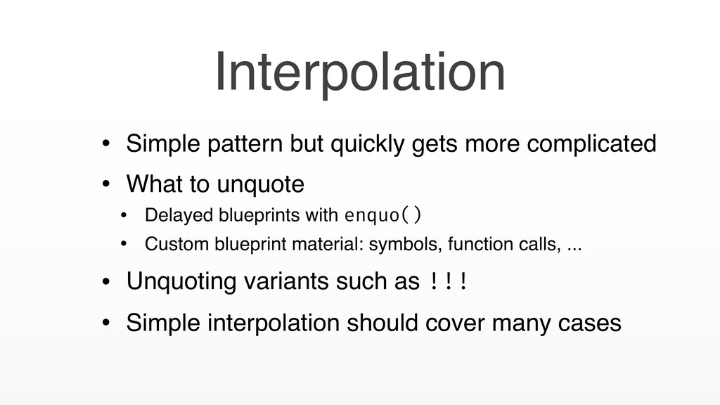
to unquote • Delayed blueprints with enquo() • Custom blueprint material: symbols, function calls, ... • Unquoting variants such as !!! • Simple interpolation should cover many cases Interpolation
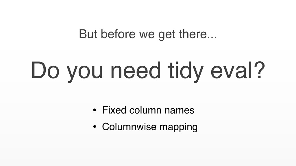
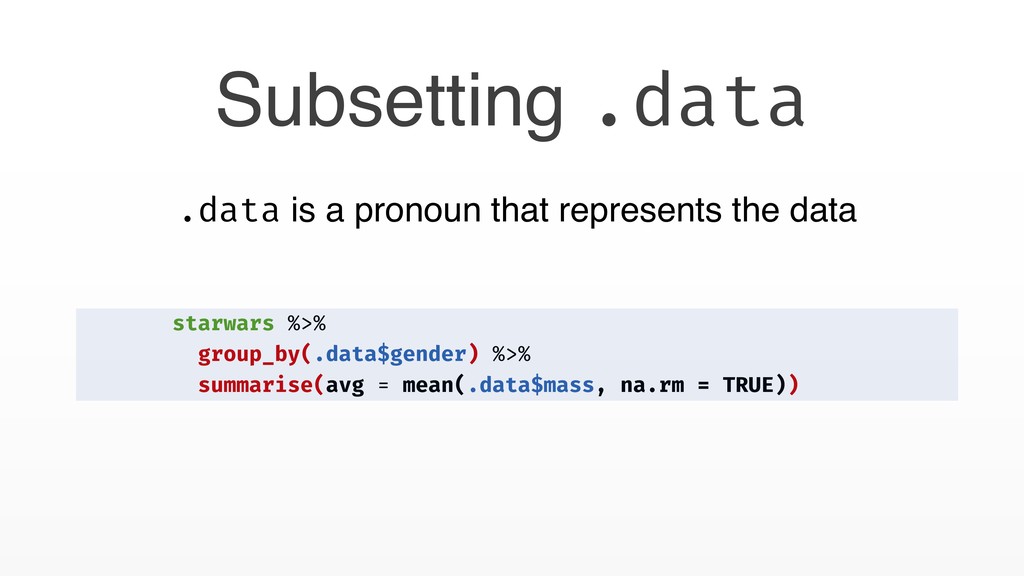
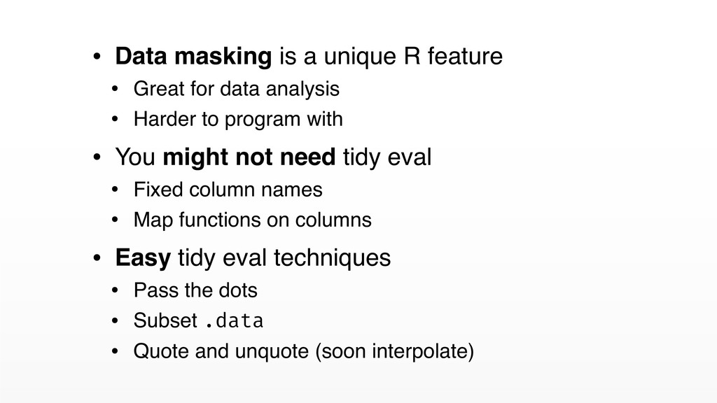
for data analysis • Harder to program with • You might not need tidy eval • Fixed column names • Map functions on columns • Easy tidy eval techniques • Pass the dots • Subset .data • Quote and unquote (soon interpolate)
![starwars[starwars$height < 200 & starwars$gender == "male", ] starwars %>%](https://files.speakerdeck.com/presentations/e61b09717bb24e659ad1b3215466e202/slide_18.jpg)
![map() loops a function automatically map(data, n_distinct) $group [1] 3](https://files.speakerdeck.com/presentations/e61b09717bb24e659ad1b3215466e202/slide_51.jpg)
![starwars %>% select(ends_with("color")) starwars %>% select(matches("^[nm]a") starwars %>% select(10, everything())](https://files.speakerdeck.com/presentations/e61b09717bb24e659ad1b3215466e202/slide_77.jpg)
![my_average <- function(data, grp_var, avg_var) { data %>% group_by(.data[[grp_var]]) %>%](https://files.speakerdeck.com/presentations/e61b09717bb24e659ad1b3215466e202/slide_106.jpg)