Deep Learning Book by I. Goodfellow, Y. Bengio and A. Courville OIST Deep Learning Reading Group Makoto Otsuka 2016-08-26 Fri Makoto Otsuka Chapter 20: Deep Generative Models
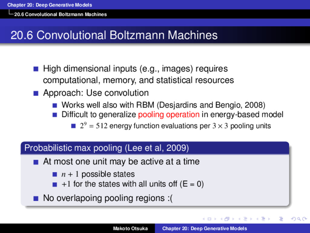
Convolutional Boltzmann Machines High dimensional inputs (e.g., images) requires computational, memory, and statistical resources Approach: Use convolution Works well also with RBM (Desjardins and Bengio, 2008) Difficult to generalize pooling operation in energy-based model 29 = 512 energy function evaluations per 3 × 3 pooling units Probabilistic max pooling (Lee et al, 2009) At most one unit may be active at a time n + 1 possible states +1 for the states with all units off (E = 0) No overlapoing pooling regions :( Makoto Otsuka Chapter 20: Deep Generative Models
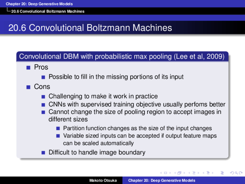
Convolutional Boltzmann Machines Convolutional DBM with probabilistic max pooling (Lee et al, 2009) Pros Possible to fill in the missing portions of its input Cons Challenging to make it work in practice CNNs with supervised training objective usually perfoms better Cannot change the size of pooling region to accept images in different sizes Partition function changes as the size of the input changes Variable sized inputs can be accepted if output feature maps can be scaled automatically Difficult to handle image boundary Makoto Otsuka Chapter 20: Deep Generative Models
or Sequential Outputs 20.7 Boltzmann Machine for Structured or Sequential Outputs Tools for modeling structured ouput can be used for modeling sequences Conditional RBM (Taylor et al., 2007) Conditional RBM + spectral hashing (Mnih et al., 2011) Factored conditional RBM for modeling motion style (Taylor and Hinton, 2009) RTRBM (Sutskever, Hinton, Taylor, 2009) RNN-RBM for learning musical notes (Boulanger-Lewandowski et al., 2012) Makoto Otsuka Chapter 20: Deep Generative Models
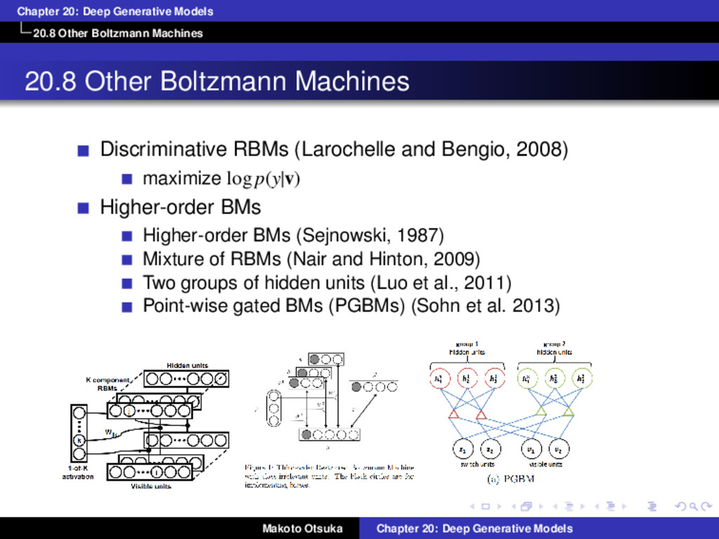
Other Boltzmann Machines Discriminative RBMs (Larochelle and Bengio, 2008) maximize log p(y|v) Higher-order BMs Higher-order BMs (Sejnowski, 1987) Mixture of RBMs (Nair and Hinton, 2009) Two groups of hidden units (Luo et al., 2011) Point-wise gated BMs (PGBMs) (Sohn et al. 2013) Makoto Otsuka Chapter 20: Deep Generative Models
20.9 Back-Propagation through Random Operations x: input variable z: simple distribution (e.g., uniform, Gaussian) f(x, z) appears stochastic If f is continuous and differentiable, we can apply BP as usual Makoto Otsuka Chapter 20: Deep Generative Models
Example: Drawing samples from a Gaussian distribution It seems counter intuitive to take a derivative of the sampling process y with respect to µ or σ y ∼ N(µ, σ2) But it make sense if we rewrite this sampling process as follows: y = µ + σz, z ∼ N(0, 1) Note that z does not depend on µ nor σ µ = g1(x; θ1), σ = g2(x; θ2) Makoto Otsuka Chapter 20: Deep Generative Models
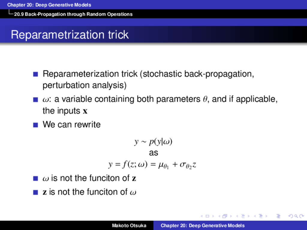
Reparametrization trick Reparameterization trick (stochastic back-propagation, perturbation analysis) ω: a variable containing both parameters θ, and if applicable, the inputs x We can rewrite y ∼ p(y|ω) as y = f(z; ω) = µθ1 + σθ2 z ω is not the funciton of z z is not the funciton of ω Makoto Otsuka Chapter 20: Deep Generative Models
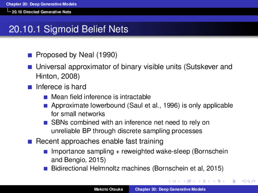
Sigmoid Belief Nets Proposed by Neal (1990) Universal approximator of binary visible units (Sutskever and Hinton, 2008) Inferece is hard Mean field inference is intractable Approximate lowerbound (Saul et al., 1996) is only applicable for small networks SBNs combined with an inference net need to rely on unreliable BP through discrete sampling processes Recent approaches enable fast training Importance sampling + reweighted wake-sleep (Bornschein and Bengio, 2015) Bidirectional Helmnoltz machines (Bornschein et al, 2015) Makoto Otsuka Chapter 20: Deep Generative Models
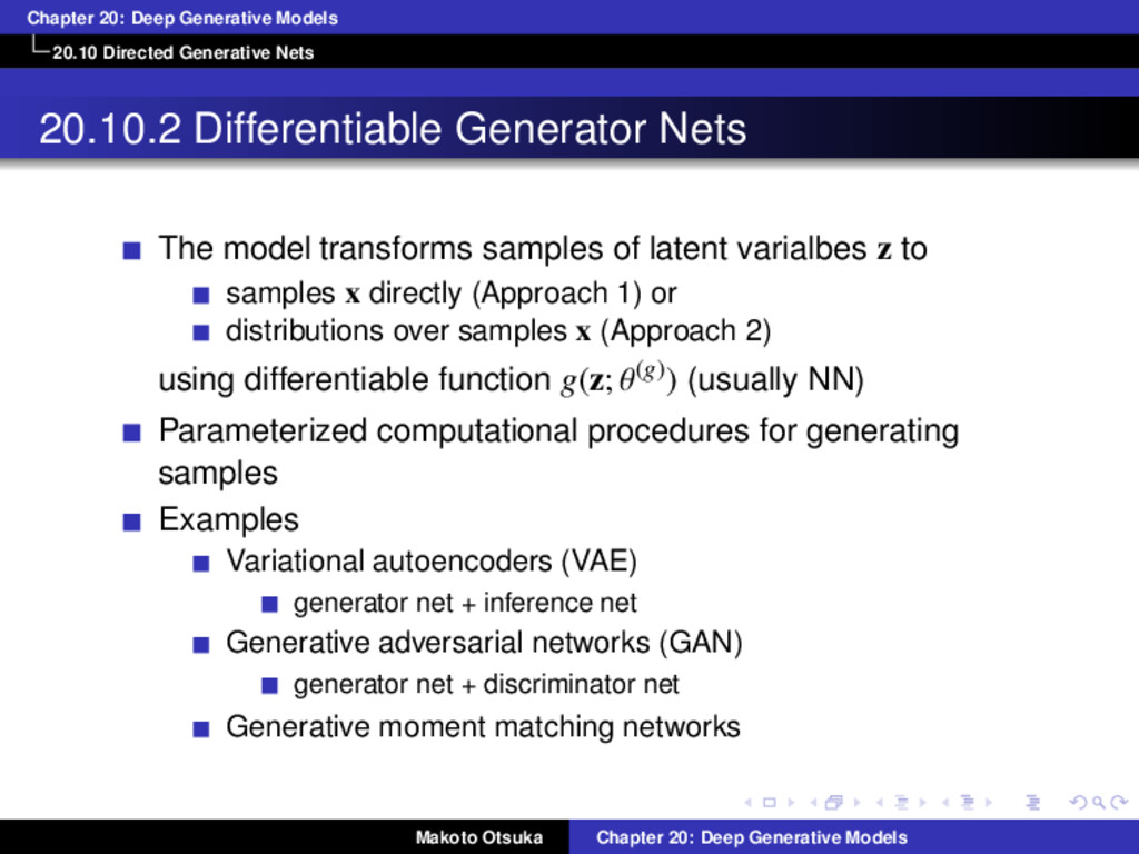
Differentiable Generator Nets The model transforms samples of latent varialbes z to samples x directly (Approach 1) or distributions over samples x (Approach 2) using differentiable function g(z; θ(g)) (usually NN) Parameterized computational procedures for generating samples Examples Variational autoencoders (VAE) generator net + inference net Generative adversarial networks (GAN) generator net + discriminator net Generative moment matching networks Makoto Otsuka Chapter 20: Deep Generative Models
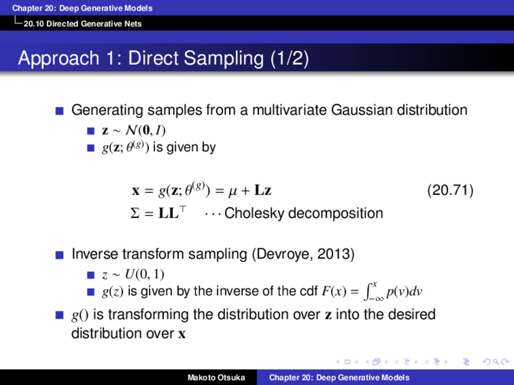
1: Direct Sampling (1/2) Generating samples from a multivariate Gaussian distribution z ∼ N(0, I) g(z; θ(g)) is given by x = g(z; θ(g)) = µ + Lz (20.71) Σ = LL⊤ · · · Cholesky decomposition Inverse transform sampling (Devroye, 2013) z ∼ U(0, 1) g(z) is given by the inverse of the cdf F(x) = ∫ x −∞ p(v)dv g() is transforming the distribution over z into the desired distribution over x Makoto Otsuka Chapter 20: Deep Generative Models
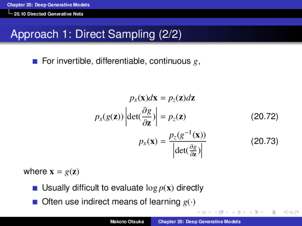
1: Direct Sampling (2/2) For invertible, differentiable, continuous g, px(x)dx = pz(z)dz px(g(z)) det( ∂g ∂z ) = pz(z) (20.72) px(x) = pz(g−1(x)) det(∂g ∂z ) (20.73) where x = g(z) Usually difficult to evaluate log p(x) directly Often use indirect means of learning g(·) Makoto Otsuka Chapter 20: Deep Generative Models
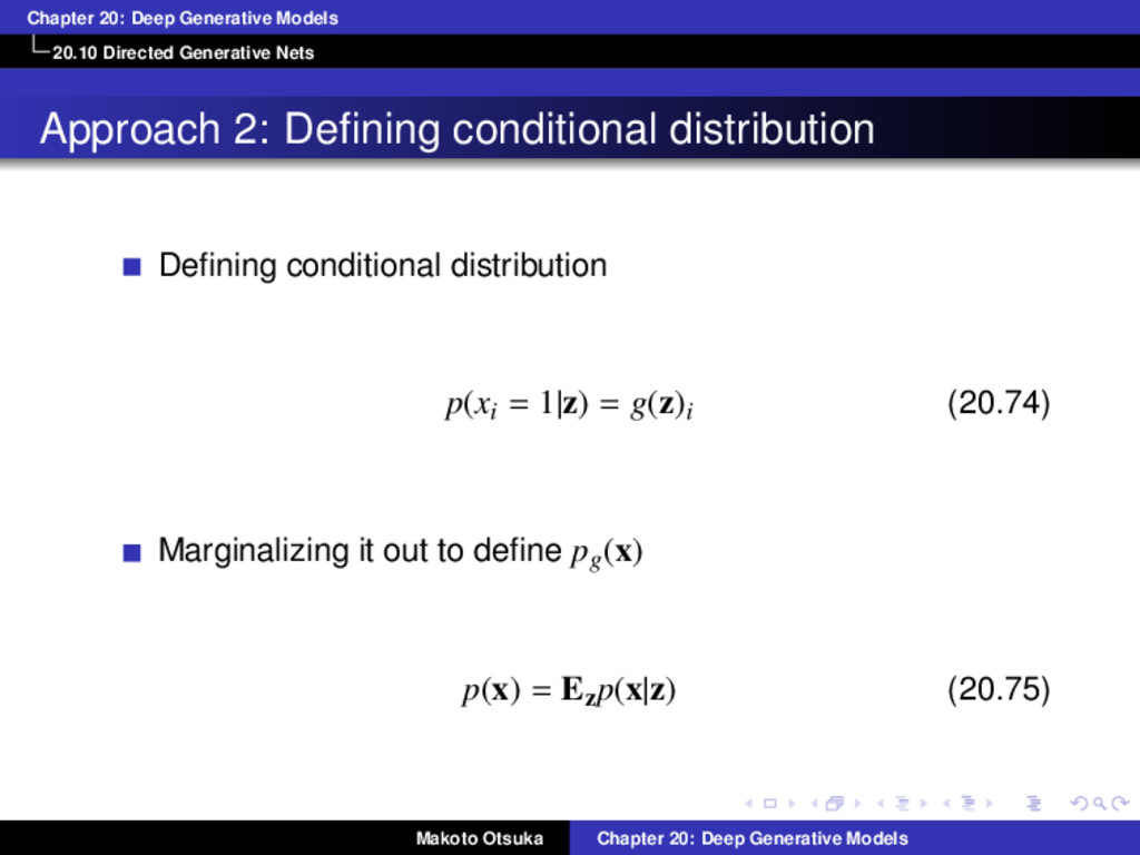
2: Defining conditional distribution Defining conditional distribution p(xi = 1|z) = g(z)i (20.74) Marginalizing it out to define pg(x) p(x) = Ezp(x|z) (20.75) Makoto Otsuka Chapter 20: Deep Generative Models
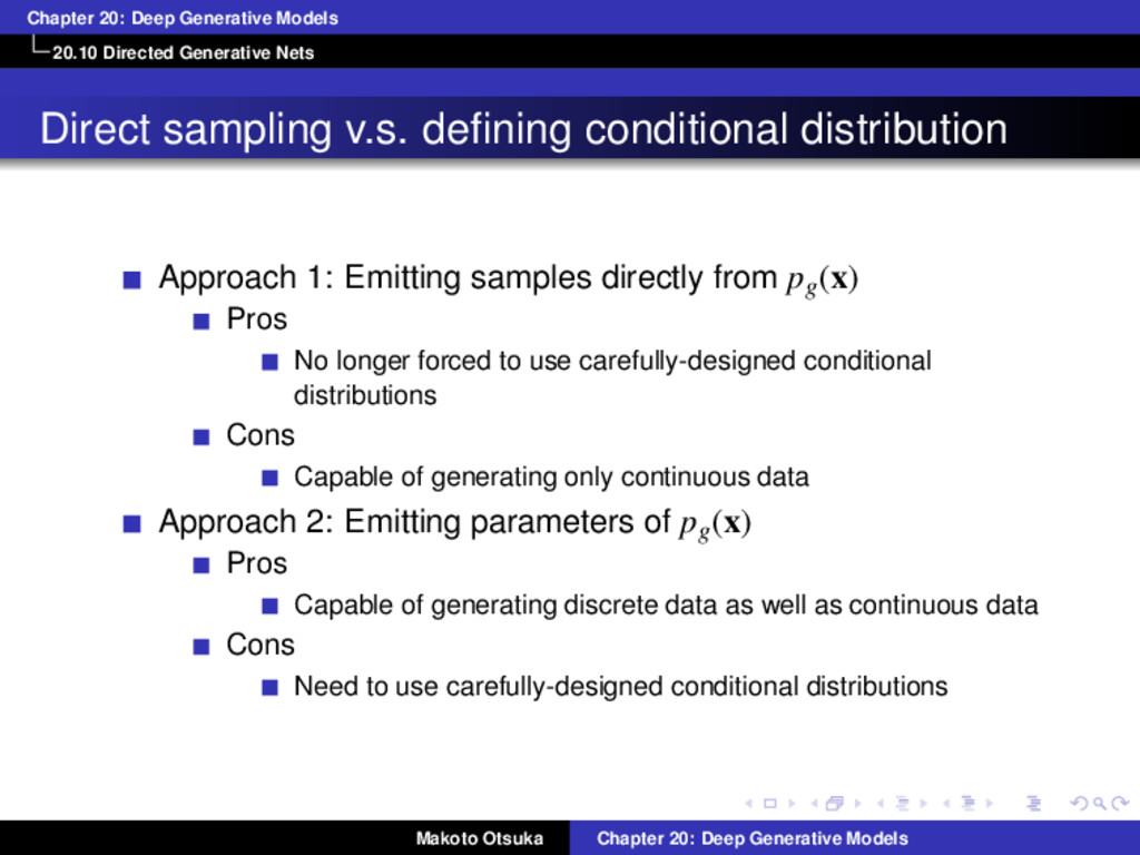
sampling v.s. defining conditional distribution Approach 1: Emitting samples directly from pg(x) Pros No longer forced to use carefully-designed conditional distributions Cons Capable of generating only continuous data Approach 2: Emitting parameters of pg(x) Pros Capable of generating discrete data as well as continuous data Cons Need to use carefully-designed conditional distributions Makoto Otsuka Chapter 20: Deep Generative Models
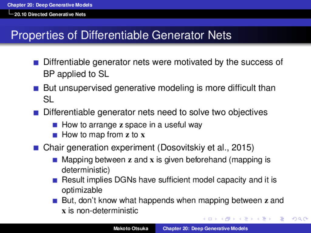
of Differentiable Generator Nets Diffrentiable generator nets were motivated by the success of BP applied to SL But unsupervised generative modeling is more difficult than SL Differentiable generator nets need to solve two objectives How to arrange z space in a useful way How to map from z to x Chair generation experiment (Dosovitskiy et al., 2015) Mapping between z and x is given beforehand (mapping is deterministic) Result implies DGNs have sufficient model capacity and it is optimizable But, don’t know what happends when mapping between z and x is non-deterministic Makoto Otsuka Chapter 20: Deep Generative Models
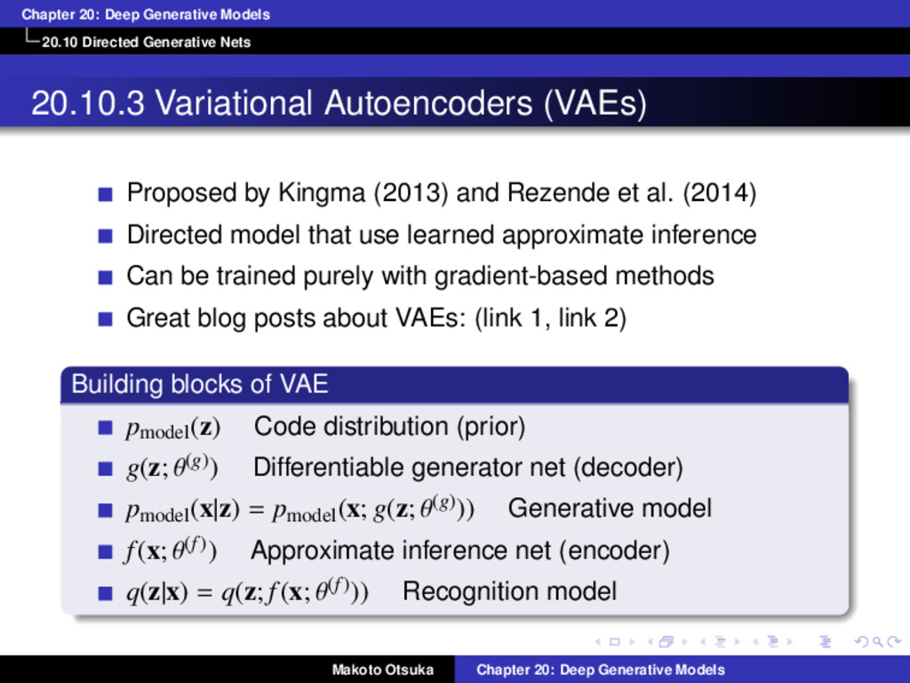
Variational Autoencoders (VAEs) Proposed by Kingma (2013) and Rezende et al. (2014) Directed model that use learned approximate inference Can be trained purely with gradient-based methods Great blog posts about VAEs: (link 1, link 2) Building blocks of VAE pmodel(z) Code distribution (prior) g(z; θ(g)) Differentiable generator net (decoder) pmodel(x|z) = pmodel(x; g(z; θ(g))) Generative model f(x; θ(f)) Approximate inference net (encoder) q(z|x) = q(z; f(x; θ(f))) Recognition model Makoto Otsuka Chapter 20: Deep Generative Models
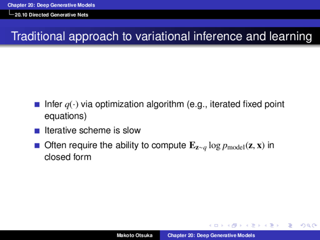
approach to variational inference and learning Infer q(·) via optimization algorithm (e.g., iterated fixed point equations) Iterative scheme is slow Often require the ability to compute Ez∼q log pmodel(z, x) in closed form Makoto Otsuka Chapter 20: Deep Generative Models
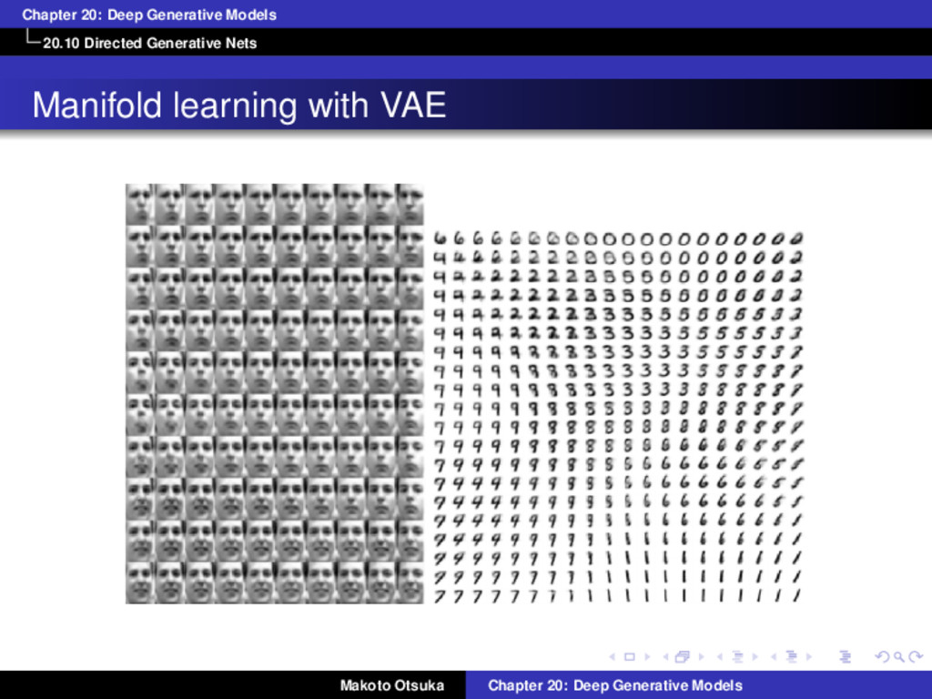
idea behind VAE Train a parameteric encoder f(x; θ(f)) for q(z|x) = q(z; f(x; θ(f))) If z is continuous, we can use BP All the expectation in L may be approximated by MC sampling Makoto Otsuka Chapter 20: Deep Generative Models
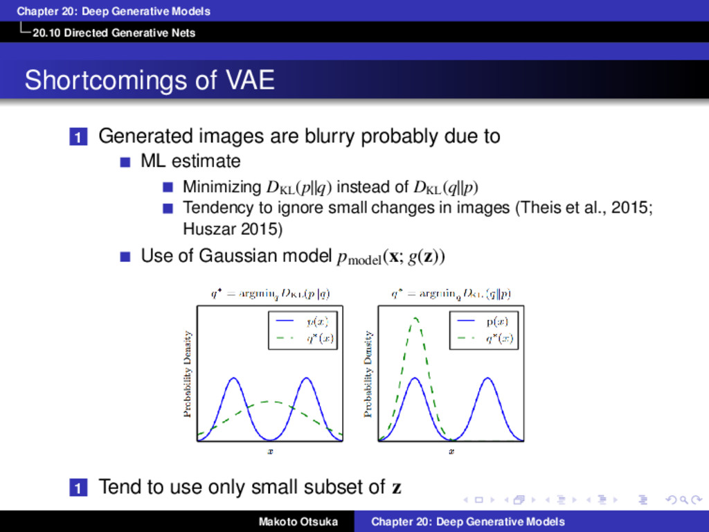
of VAE 1 Generated images are blurry probably due to ML estimate Minimizing DKL (p||q) instead of DKL (q||p) Tendency to ignore small changes in images (Theis et al., 2015; Huszar 2015) Use of Gaussian model pmodel(x; g(z)) 1 Tend to use only small subset of z Makoto Otsuka Chapter 20: Deep Generative Models
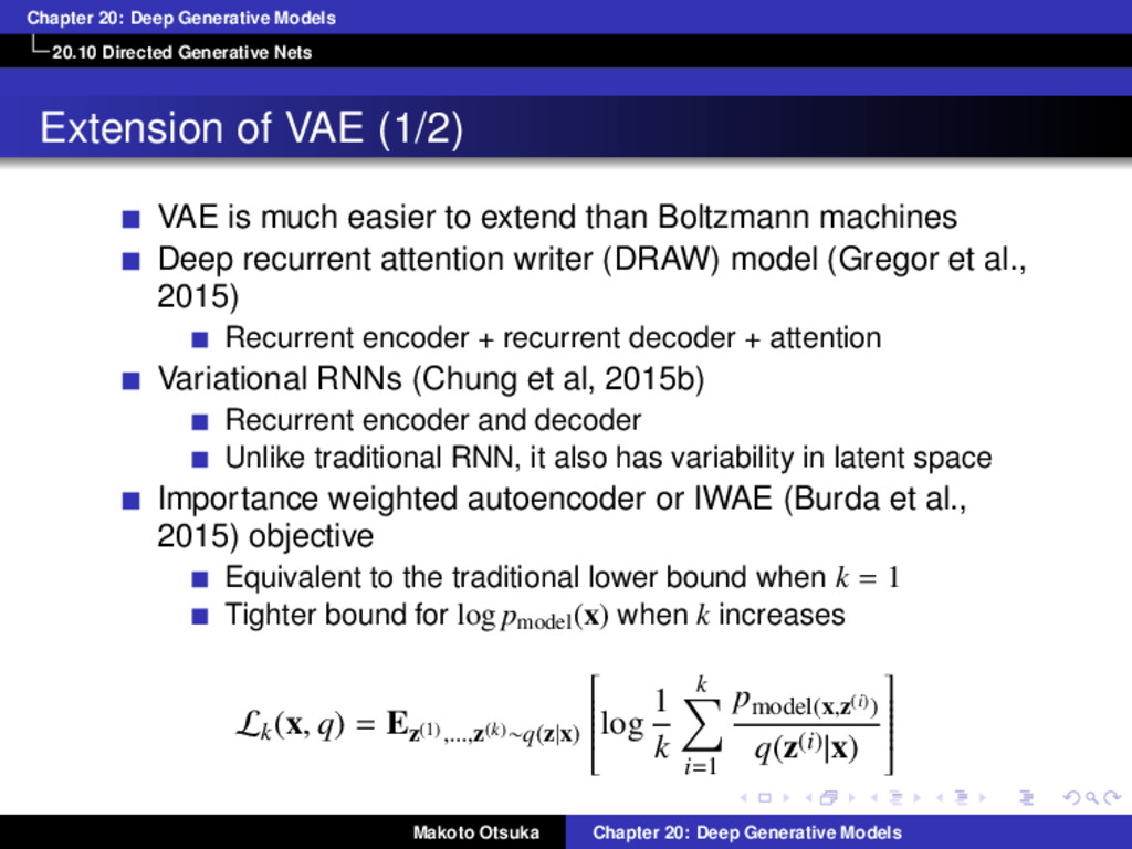
of VAE (1/2) VAE is much easier to extend than Boltzmann machines Deep recurrent attention writer (DRAW) model (Gregor et al., 2015) Recurrent encoder + recurrent decoder + attention Variational RNNs (Chung et al, 2015b) Recurrent encoder and decoder Unlike traditional RNN, it also has variability in latent space Importance weighted autoencoder or IWAE (Burda et al., 2015) objective Equivalent to the traditional lower bound when k = 1 Tighter bound for log pmodel(x) when k increases Lk(x, q) = Ez(1),...,z(k)∼q(z|x) log 1 k k ∑ i=1 pmodel(x,z(i)) q(z(i)|x) Makoto Otsuka Chapter 20: Deep Generative Models
of VAE (2/2) Some interesting connections to the multi-prediction DBM (MP-DBM) in Fig. 20.5 and other approaches that involve back-propagation through the approximate inference graph (Goodfellow et al., 2013b; Stoyanov et al., 2011; Brakel et al., 2013). VAE is defined for arbitrary computational graphs No need to restrict the choice of models to those with tractable mean field fixed point equations One disadvantage of the variational autoencoder is that it learns an inference network for only one problem, inferring z given x. Makoto Otsuka Chapter 20: Deep Generative Models
Generative Adversarial Networks (GANs) Proposed by Goodfellow et al. (2014c) Example of differentiable generator networks Generator net: g(z; θ(g)) Directly produces samples: x = g(z; θ(g)) Payoff is −v(θ(g), θ(d)) Attempts to fool the classifier into believing its samples are real Discriminator net: d(x; θ(d)) (probability of x being real) Payoff is v(θ(g), θ(d)) Attempts to learn to correctly classify samples as real or fake g∗ = arg min g max d v(g, d) v(θ(g), θ(d)) = Ex∼pdata log d(x) + Ex∼pmodel log(1 − d(x)) Makoto Otsuka Chapter 20: Deep Generative Models
in GANs Learning is difficult in GAN E.g.) v(a, b) = ab Note that the equilibria for a minimax game are not local minima of v Instead, they are points that are simultaneously minima for both players’ costs. This means that they are saddle points of v that are local minima with respect to the first player’s parameters and local maxima with respect to the second player’s parameters. Alternative formulation of payoffs (Goodfellow et al., 2014c) Makoto Otsuka Chapter 20: Deep Generative Models
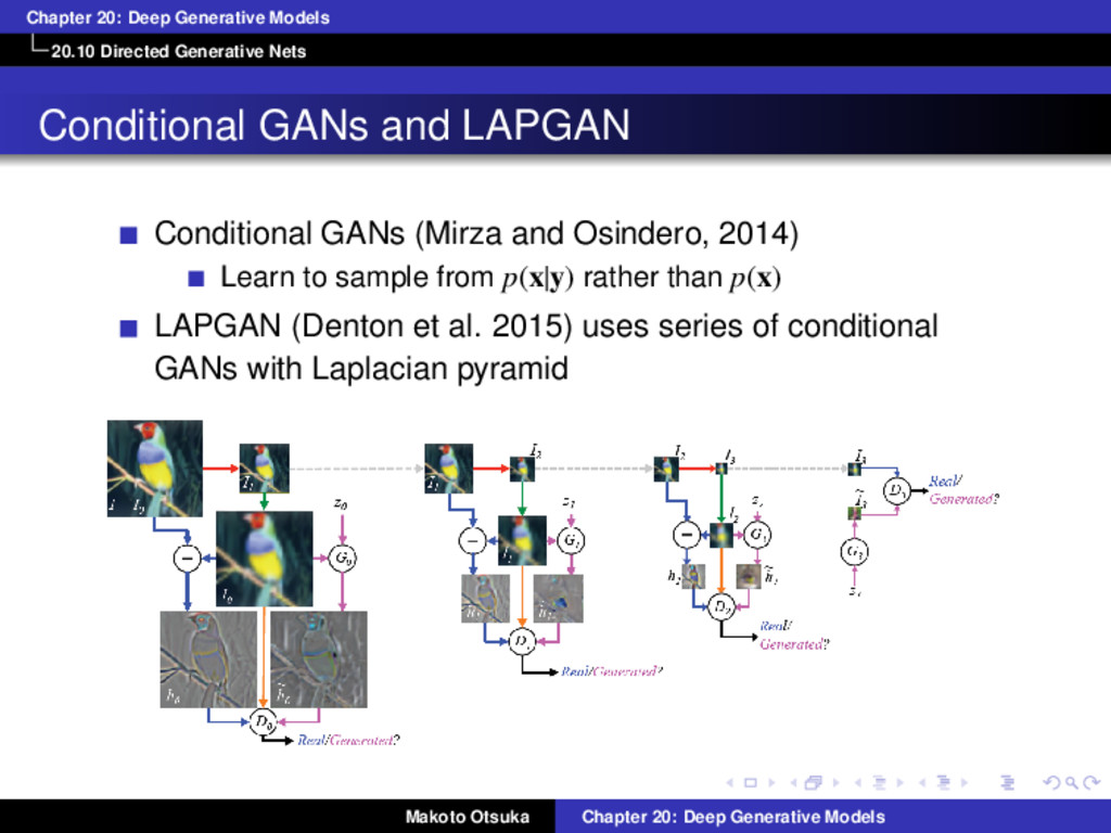
GANs and LAPGAN Conditional GANs (Mirza and Osindero, 2014) Learn to sample from p(x|y) rather than p(x) LAPGAN (Denton et al. 2015) uses series of conditional GANs with Laplacian pyramid Makoto Otsuka Chapter 20: Deep Generative Models
of GAN It can fit distribution that assign zero probability to the training points. Somehow tracing out manifold that is spanned by training data Add Gaussian noise to all of the generated values to ensure non-zero probabilities to all points Dropout seems to be important in the discriminator network In particular, units should be stochastically dropped while computing the gradient for the generator network to follow. Makoto Otsuka Chapter 20: Deep Generative Models
similar to GAN GAN is designed for differentiable generator net. Similar principles can be used to train other kind of models Self-supervised boosting can be used to train RBM generator to fool a logistic regression discriminator (Welling et al., 2002) Makoto Otsuka Chapter 20: Deep Generative Models
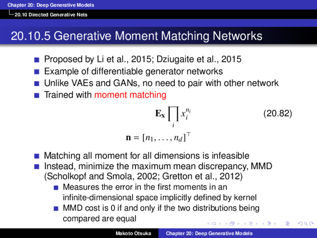
Generative Moment Matching Networks Proposed by Li et al., 2015; Dziugaite et al., 2015 Example of differentiable generator networks Unlike VAEs and GANs, no need to pair with other network Trained with moment matching Ex ∏ i xni i (20.82) n = [n1 , . . . , nd]⊤ Matching all moment for all dimensions is infeasible Instead, minimize the maximum mean discrepancy, MMD (Scholkopf and Smola, 2002; Gretton et al., 2012) Measures the error in the first moments in an infinite-dimensional space implicitly defined by kernel MMD cost is 0 if and only if the two distributions being compared are equal Makoto Otsuka Chapter 20: Deep Generative Models
Moment Matching Networks Samples from GMMN is not visually pleasing Visual can be improved if generator is combined with an autoencoder Need large batch size to obtain reliable estimate of the moment Makoto Otsuka Chapter 20: Deep Generative Models
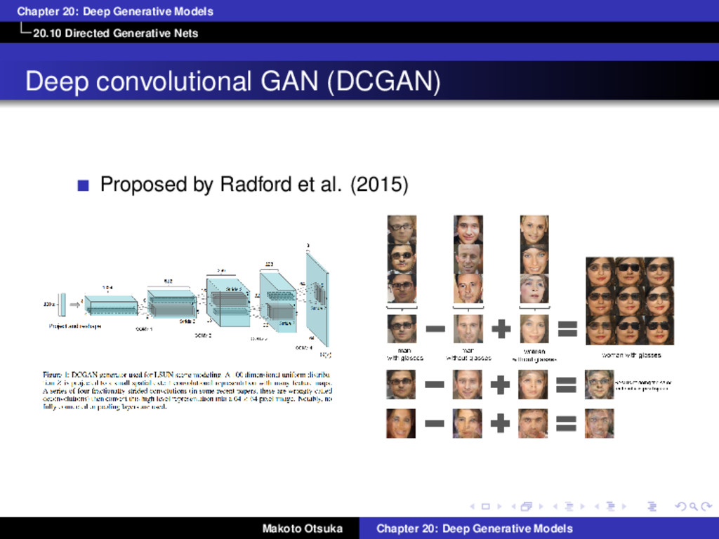
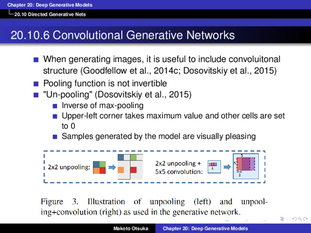
Convolutional Generative Networks When generating images, it is useful to include convoluitonal structure (Goodfellow et al., 2014c; Dosovitskiy et al., 2015) Pooling function is not invertible "Un-pooling" (Dosovitskiy et al., 2015) Inverse of max-pooling Upper-left corner takes maximum value and other cells are set to 0 Samples generated by the model are visually pleasing Makoto Otsuka Chapter 20: Deep Generative Models
Auto-Regressive Networks Directed probabilistic models with no latent random variables Fully-visible Bayes networks (FVBNs) NADE (Larochelle and Murray, 2011) One type of auto-regressive network Reuse of features Statistical advantages (fewer unique parameters) Computational advantages (less computation) Makoto Otsuka Chapter 20: Deep Generative Models
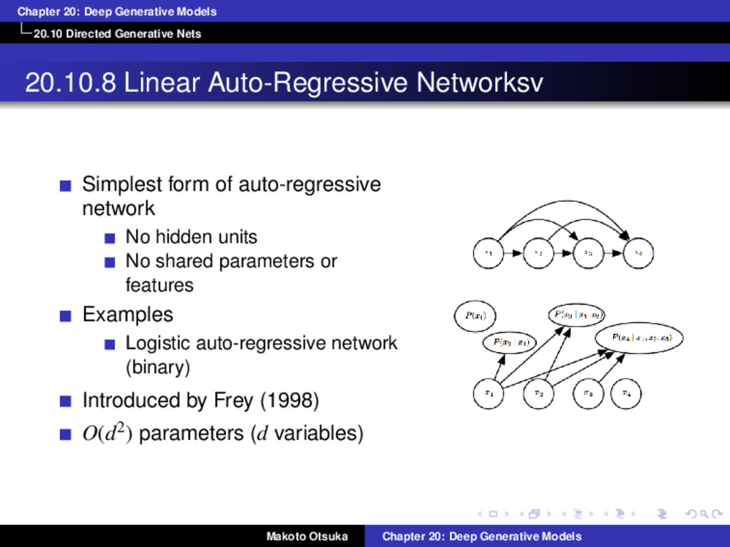
Linear Auto-Regressive Networksv Simplest form of auto-regressive network No hidden units No shared parameters or features Examples Logistic auto-regressive network (binary) Introduced by Frey (1998) O(d2) parameters (d variables) Makoto Otsuka Chapter 20: Deep Generative Models
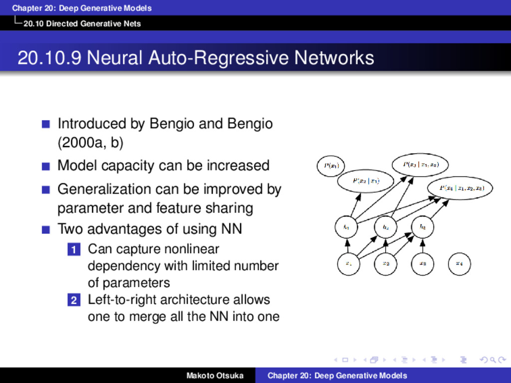
Neural Auto-Regressive Networks Introduced by Bengio and Bengio (2000a, b) Model capacity can be increased Generalization can be improved by parameter and feature sharing Two advantages of using NN 1 Can capture nonlinear dependency with limited number of parameters 2 Left-to-right architecture allows one to merge all the NN into one Makoto Otsuka Chapter 20: Deep Generative Models
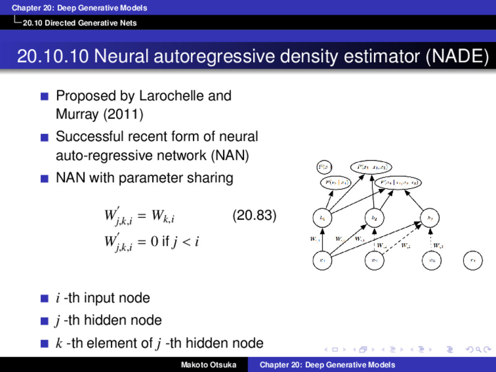
Neural autoregressive density estimator (NADE) Proposed by Larochelle and Murray (2011) Successful recent form of neural auto-regressive network (NAN) NAN with parameter sharing W′ j,k,i = Wk,i (20.83) W′ j,k,i = 0 if j < i i -th input node j -th hidden node k -th element of j -th hidden node Makoto Otsuka Chapter 20: Deep Generative Models
of NADE NADE-k (Raiko et al, 2014) k-step mean field recurrent inference RNADE (Uria et al., 2013) Processing continuous-valued data using Gaussian mixture Use pseudo-gradient to reduce unstable gradient calculation caused by coupling of µi and σ2 i Ensemble of NADE models handling reordered inputs o (Murray and Larochelle, 2014) Better generalization than a fixed-order model pensemble(x) = 1 k k ∑ i=1 p(x|o(i)) Deep NADE is computationally expensive and not so much gain Makoto Otsuka Chapter 20: Deep Generative Models
20.11 Drawing Samples from Autoencoders Underlying connections between score matching, denoising autoencoders, and contractive autoencoders They are learning data distributions, but how can we sample data? VAE - ancestral sampling CAE Repeated encoding and decoding with injected noise will induce a random walk along the surface of the manifold (Rifai et al., 2012; Mesnil et al., 2012) Manifold diffusion technique (kind of MC) DAE More general MC Makoto Otsuka Chapter 20: Deep Generative Models
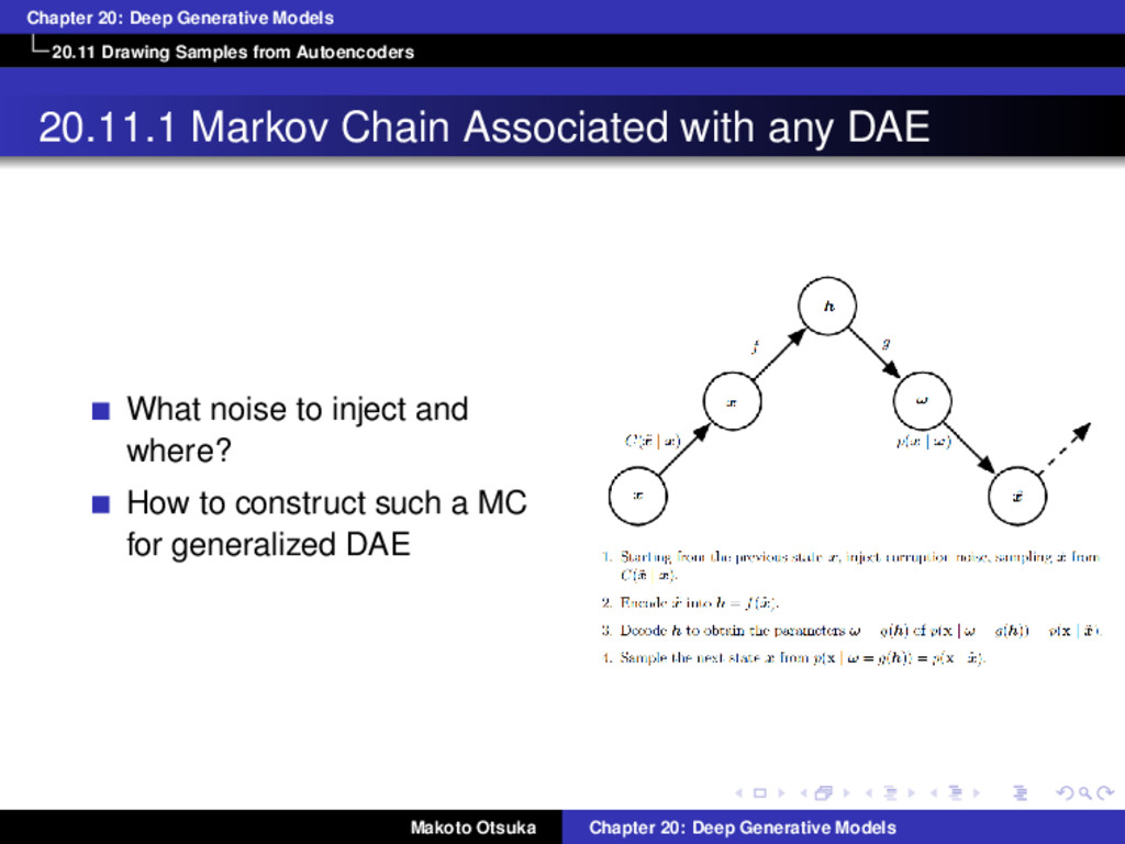
20.11.1 Markov Chain Associated with any DAE What noise to inject and where? How to construct such a MC for generalized DAE Makoto Otsuka Chapter 20: Deep Generative Models
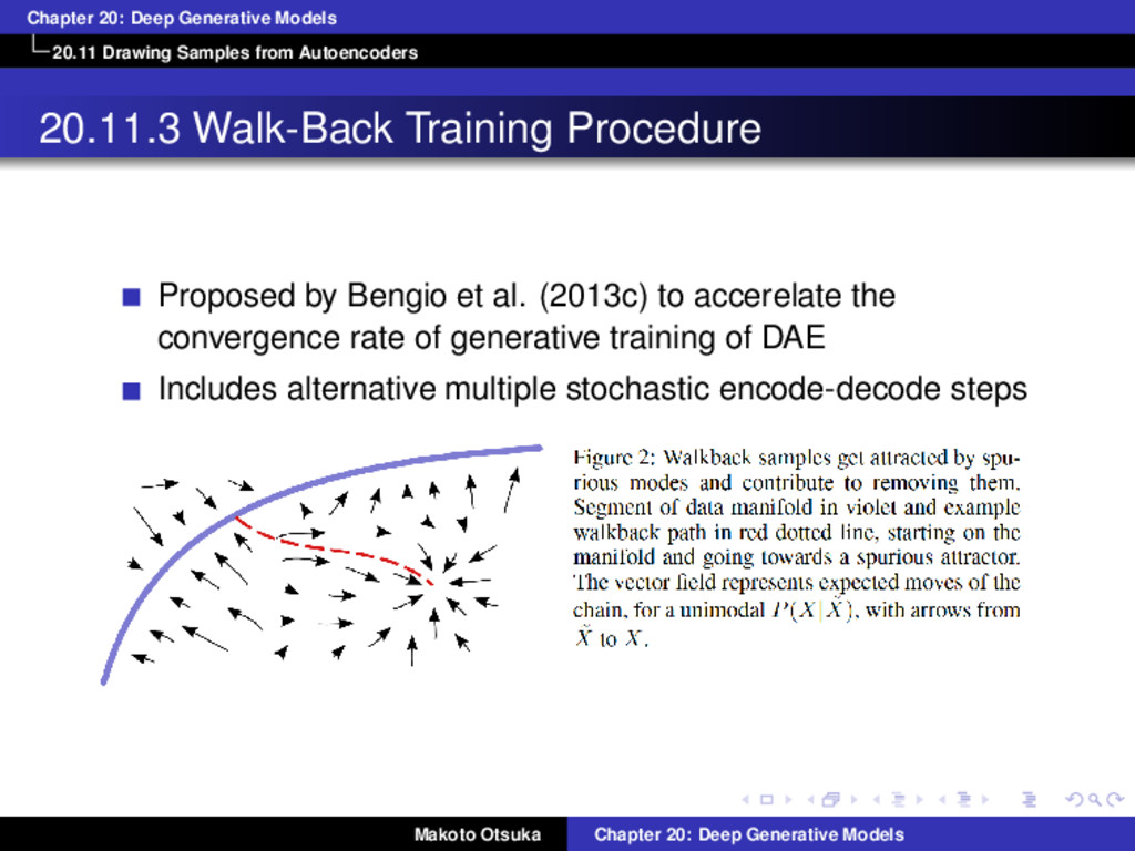
20.11.3 Walk-Back Training Procedure Proposed by Bengio et al. (2013c) to accerelate the convergence rate of generative training of DAE Includes alternative multiple stochastic encode-decode steps Makoto Otsuka Chapter 20: Deep Generative Models
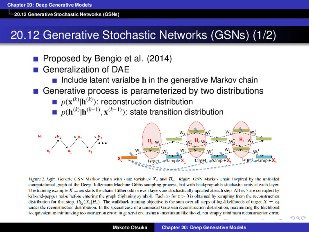
20.12 Generative Stochastic Networks (GSNs) (1/2) Proposed by Bengio et al. (2014) Generalization of DAE Include latent varialbe h in the generative Markov chain Generative process is parameterized by two distributions p(x(k)|h(k)): reconstruction distribution p(h(k)|h(k−1), x(k−1)): state transition distribution Makoto Otsuka Chapter 20: Deep Generative Models
20.12 Generative Stochastic Networks (GSNs) (2/2) Properties of GSNs Joint distribution is defined implicitly by MC if it exists Maximize log p(x(k) = x|h(k)) where x(0) = x Walk-back training protocol was used to improve training convergence 20.12.1 Discriminant GSNs Possible to model p(y|x) instead of p(x) with GSNs Makoto Otsuka Chapter 20: Deep Generative Models
Other Generation Schemes So far, MCMC sampling, ancestral sampling, or some mixture of the two Diffusion inversion objective for learning a generative model based on non-equilibrium thermodynamics (Sohl-Dickstein et al., 2015) Structured -> unstructured Running this process backward Approximate Bayesian computation (ABC) framework (Rubin et al., 1984) Samples are rejected or modified in order to make the moments of selected functions of the samples match those of the desired distribution. This is not a moment matching because ABC changes the samples themselves Makoto Otsuka Chapter 20: Deep Generative Models
Evaluating Generative Models (1/2) Usually we cannot evaluate log p(x) directly Which is better? Stochastic estimate of the log-likelihood for model A Deterministic lower bound on the log-likelihood for model B High likelihood estimate log p(x) = log ˜ p(x) − log Z can be obtained due to Good model, or Bad AIS implimentation (underestimate Z) Makoto Otsuka Chapter 20: Deep Generative Models
Evaluating Generative Models (2/2) Changing preprocessing step is unacceptable when comparing different generative models e.g., multiplying the input by 0.1 will artificially increase likelihood by a factor of 10 It is essential to compare real-valued MNIST models only to other real-valued models and binary-valued models only to other binary-valued models Use exactly same binalization scheme for all compared models Visual inspection can be used but not a reliable measure Poor model can produce good examples by overfitting Need to develop some other ways to evaluate generative models You can get extremely high likelihood by asigning arbitrarily low variance to background pixels that never changes Makoto Otsuka Chapter 20: Deep Generative Models