Introduction to Data Visualization for Meta-Analysis

Presentation slides for the Spring 2018 workshop in data visualization for PM 605: Systematic Review and Meta-Analysis.

Transcript

1. Introduction to Data Visualization for Meta- Analysis with tidymeta and ggplot2 Malcolm Barrett Install R: bit.ly/pm605_r Handout: bit.ly/pm605_tut
2. Data Visualization with R ggplot2 and the tidyverse are friendly and consistent tools for data analysis and visualization 2 / 73
3. Data Visualization with R ggplot2 and the tidyverse are friendly and consistent tools for data analysis and visualization Better plots are better communication 3 / 73
4. Data Visualization with R ggplot2 and the tidyverse are friendly and consistent tools for data analysis and visualization Better plots are better communication tidymeta makes it easy to manipulate and plot meta-analysis results 4 / 73
5. Introduction to the Data What's the impact of intrauterine device (IUD) use on risk of cervical cancer? 5 / 73
6. Introduction to the Data What's the impact of intrauterine device (IUD) use on risk of cervical cancer? 16 studies: 4,945 cases and 7,537 controls 6 / 73
7. Introduction to the Data What's the impact of intrauterine device (IUD) use on risk of cervical cancer? 16 studies: 4,945 cases and 7,537 controls Women who used IUDs were at a third less risk than those who didn't (OR 0.64) 7 / 73
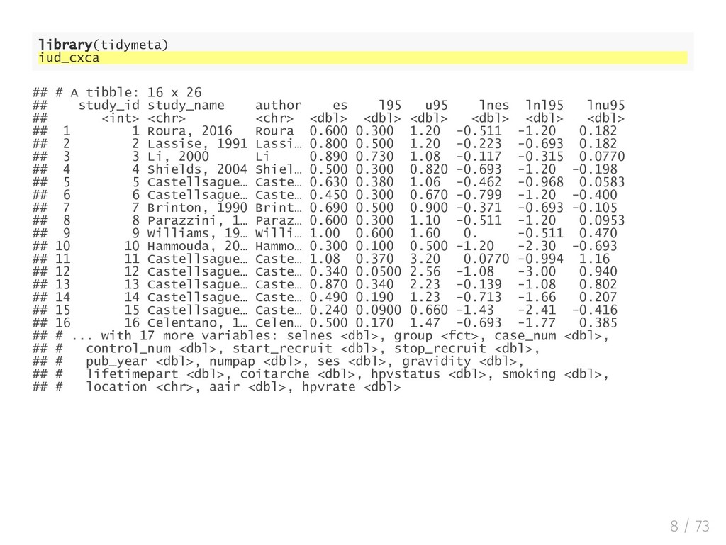
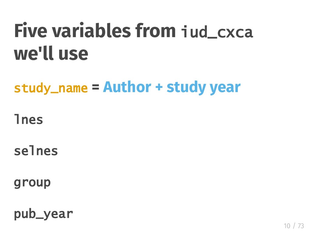
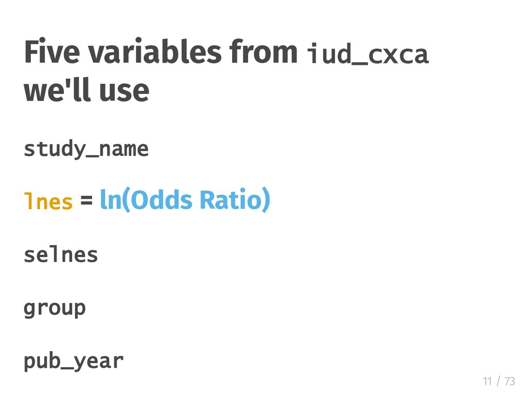
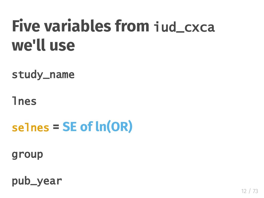
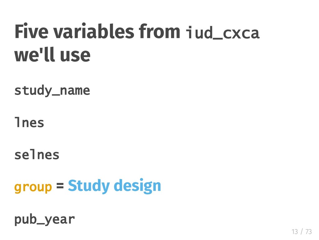
8. library(tidymeta) iud_cxca ## # A tibble: 16 x 26 ## study_id study_name author es l95 u95 lnes lnl95 lnu95 ## <int> <chr> <chr> <dbl> <dbl> <dbl> <dbl> <dbl> <dbl> ## 1 1 Roura, 2016 Roura 0.600 0.300 1.20 -0.511 -1.20 0.182 ## 2 2 Lassise, 1991 Lassi… 0.800 0.500 1.20 -0.223 -0.693 0.182 ## 3 3 Li, 2000 Li 0.890 0.730 1.08 -0.117 -0.315 0.0770 ## 4 4 Shields, 2004 Shiel… 0.500 0.300 0.820 -0.693 -1.20 -0.198 ## 5 5 Castellsague… Caste… 0.630 0.380 1.06 -0.462 -0.968 0.0583 ## 6 6 Castellsague… Caste… 0.450 0.300 0.670 -0.799 -1.20 -0.400 ## 7 7 Brinton, 1990 Brint… 0.690 0.500 0.900 -0.371 -0.693 -0.105 ## 8 8 Parazzini, 1… Paraz… 0.600 0.300 1.10 -0.511 -1.20 0.0953 ## 9 9 Williams, 19… Willi… 1.00 0.600 1.60 0. -0.511 0.470 ## 10 10 Hammouda, 20… Hammo… 0.300 0.100 0.500 -1.20 -2.30 -0.693 ## 11 11 Castellsague… Caste… 1.08 0.370 3.20 0.0770 -0.994 1.16 ## 12 12 Castellsague… Caste… 0.340 0.0500 2.56 -1.08 -3.00 0.940 ## 13 13 Castellsague… Caste… 0.870 0.340 2.23 -0.139 -1.08 0.802 ## 14 14 Castellsague… Caste… 0.490 0.190 1.23 -0.713 -1.66 0.207 ## 15 15 Castellsague… Caste… 0.240 0.0900 0.660 -1.43 -2.41 -0.416 ## 16 16 Celentano, 1… Celen… 0.500 0.170 1.47 -0.693 -1.77 0.385 ## # ... with 17 more variables: selnes <dbl>, group <fct>, case_num <dbl>, ## # control_num <dbl>, start_recruit <dbl>, stop_recruit <dbl>, ## # pub_year <dbl>, numpap <dbl>, ses <dbl>, gravidity <dbl>, ## # lifetimepart <dbl>, coitarche <dbl>, hpvstatus <dbl>, smoking <dbl>, ## # location <chr>, aair <dbl>, hpvrate <dbl> 8 / 73
9. Five variables from iud_cxca we'll use study_name lnes selnes group pub_year 9 / 73
10. Five variables from iud_cxca we'll use study_name = Author + study year lnes selnes group pub_year 10 / 73
11. Five variables from iud_cxca we'll use study_name lnes = ln(Odds Ratio) selnes group pub_year 11 / 73
12. Five variables from iud_cxca we'll use study_name lnes selnes = SE of ln(OR) group pub_year 12 / 73
13. Five variables from iud_cxca we'll use study_name lnes selnes group = Study design pub_year 13 / 73
14. Five variables from iud_cxca we'll use study_name lnes selnes group pub_year = Publication year 14 / 73
15. Meta-Analysis Plot Types 15 / 73
16. Meta-Analysis Plot Types Forest Plot 16 / 73
17. forest_plot() 17 / 73
18. Meta-Analysis Plot Types Forest Plot Funnel Plot 18 / 73
19. funnel_plot() 19 / 73
20. Meta-Analysis Plot Types Forest Plot Funnel Plot In uence/Sensitivity Plot 20 / 73
21. influence_plot() 21 / 73
22. Meta-Analysis Plot Types Forest Plot Funnel Plot In uence/Sensitivity Plot Cumulative Plot 22 / 73
23. cumulative_plot() 23 / 73
24. A Crash Course in the Tidyverse 24 / 73
25. ggplot2: Elegant Data Visualizations in R 25 / 73
26. ggplot2: Elegant Data Visualizations in R Based on a Grammar of Graphics 26 / 73
27. ggplot2: Elegant Data Visualizations in R Based on a Grammar of Graphics Data is mapped to aesthetics; Statistics and plot are linked 27 / 73
28. ggplot2: Elegant Data Visualizations in R Based on a Grammar of Graphics Data is mapped to aesthetics; Statistics and plot are linked Sensible defaults; In nitely extensible 28 / 73
29. library(ggplot2) p <- ggplot(iud_cxca, aes(case_num + control_num, lnes, color = group)) p 29 / 73
30. library(ggplot2) p <- p + geom_point() p 30 / 73
31. p <- p + geom_smooth(method = "lm", se = FALSE) p 31 / 73
32. p + labs(title = "The Effect of Sample Size on Estimate", x = "Sample Size", y = "ln(Odds Ratio)") + scale_color_discrete(name = "Study Design") + theme_minimal() + theme(text = element_text(size = 16)) 32 / 73
33. Tidy Data is Easier to Plot 33 / 73
34. Tidy Data is Easier to Plot Each column is a single variable 34 / 73
35. Tidy Data is Easier to Plot Each column is a single variable Each row is a single observation 35 / 73
36. Tidy Data is Easier to Plot Each column is a single variable Each row is a single observation Each cell is a value 36 / 73
37. %>% mutate() arrange() group_by() tidy() Our Tidy Tools 37 / 73
38. %>%: passes the results of one function to the next mutate() arrange() group_by() tidy() Our Tidy Tools 38 / 73
39. %>% mutate(): changes or creates a new variable arrange() group_by() tidy() Our Tidy Tools 39 / 73
40. %>% mutate() arrange(): sorts a data set by a variable group_by() tidy() Our Tidy Tools 40 / 73
41. %>% mutate() arrange() group_by(): groups a data set by a variable tidy() Our Tidy Tools 41 / 73
42. %>% mutate() arrange() group_by() tidy(): tidies statistical results Our Tidy Tools 42 / 73
43. Tidy Meta-Analysis meta_analysis() 43 / 73
44. Tidy Meta-Analysis meta_analysis() ma <- iud_cxca %>% group_by(group) %>% meta_analysis(yi = lnes, sei = selnes, slab = study_name, exponentiate = TRUE) ma ## # A tibble: 21 x 11 ## group study type estimate std.error statistic p.value conf.low ## <fct> <chr> <chr> <dbl> <dbl> <dbl> <dbl> <dbl> ## 1 Nested … Roura, 2… study 0.600 0.354 -1.44 NA 0.300 ## 2 Nested … Subgroup… summ… 0.600 0.354 -1.44 0.149 0.300 ## 3 Populat… Lassise,… study 0.800 0.223 -0.999 NA 0.516 ## 4 Populat… Li, 2000 study 0.890 0.0999 -1.17 NA 0.732 ## 5 Populat… Shields,… study 0.500 0.257 -2.70 NA 0.302 ## 6 Populat… Castells… study 0.630 0.262 -1.77 NA 0.377 ## 7 Populat… Castells… study 0.450 0.205 -3.90 NA 0.301 ## 8 Populat… Subgroup… summ… 0.655 0.146 -2.90 0.00374 0.492 ## 9 Clinic-… Brinton,… study 0.690 0.150 -2.47 NA 0.514 ## 10 Clinic-… Parazzin… study 0.600 0.331 -1.54 NA 0.313 ## # ... with 11 more rows, and 3 more variables: conf.high <dbl>, ## # meta <list>, weight <dbl> 44 / 73
45. Forest Plot forest_plot() 45 / 73
46. Forest Plot forest_plot() ma %>% forest_plot(group = group) 46 / 73
47. Forest Plot forest_plot() ma %>% forest_plot(group = group) text_table() 47 / 73
48. Forest Plot forest_plot() ma %>% forest_plot(group = group) text_table() ma %>% text_table(group = group, "Weights" = weight) 48 / 73
49. patchwork: Compose ggplots 49 / 73
50. Join ggplots quickly and accurately patchwork: Compose ggplots 50 / 73
51. Join ggplots quickly and accurately library(patchwork) forest_plot() + text_table() patchwork: Compose ggplots 51 / 73
52. Funnel Plot funnel_plot() 52 / 73
53. Funnel Plot funnel_plot() ma %>% funnel_plot(log_summary = TRUE) 53 / 73
54. In uence Plot sensitivity() 54 / 73
55. In uence Plot sensitivity() ma %>% sensitivity(exponentiate = TRUE) 55 / 73
56. In uence Plot sensitivity() ma %>% sensitivity(exponentiate = TRUE) influence_plot() 56 / 73
57. In uence Plot sensitivity() ma %>% sensitivity(exponentiate = TRUE) influence_plot() ma %>% sensitivity(exponentiate = TRUE) %>% influence_plot() 57 / 73
58. Cumulative Plot cumulative() 58 / 73
59. Cumulative Plot cumulative() ma %>% arrange(desc(weight)) %>% cumulative(exponentiate = TRUE) 59 / 73
60. Cumulative Plot cumulative() ma %>% arrange(desc(weight)) %>% cumulative(exponentiate = TRUE) cumulative_plot() 60 / 73
61. Cumulative Plot cumulative() ma %>% arrange(desc(weight)) %>% cumulative(exponentiate = TRUE) cumulative_plot() ma %>% arrange(desc(weight)) %>% cumulative(exponentiate = TRUE) %>% cumulative_plot(sum_lines = FALSE) 61 / 73
62. Importing Stata data, saving ggplots 62 / 73
63. Importing Stata data, saving ggplots haven: read_dta() 63 / 73
64. Importing Stata data, saving ggplots haven: read_dta() library(haven) data <- read_dta("stata_data.dta") 64 / 73
65. Importing Stata data, saving ggplots haven: read_dta() library(haven) data <- read_dta("stata_data.dta") ggplot2: ggsave() 65 / 73
66. Importing Stata data, saving ggplots haven: read_dta() library(haven) data <- read_dta("stata_data.dta") ggplot2: ggsave() library(ggplot2) p <- forest_plot(ma, group = group) ggsave(p, "forest_plot.png", dpi = 320, height = 8) 66 / 73
67. tidymeta 67 / 73
68. tidymeta meta_analysis()/your_favorite_function() + tidy() 68 / 73
69. tidymeta meta_analysis()/your_favorite_function() + tidy() forest_plot()/text_table() 69 / 73
70. tidymeta meta_analysis()/your_favorite_function() + tidy() forest_plot()/text_table() sensitivity()/influence_plot() 70 / 73
71. tidymeta meta_analysis()/your_favorite_function() + tidy() forest_plot()/text_table() sensitivity()/influence_plot() cumulative()/cumulative_plot() 71 / 73
72. Resources R for Data Science: A comprehensive but friendly introduction to the tidyverse. Free online. DataCamp: ggplot2 courses and tidyverse courses ggplot2: Elegant Graphics for Data Analysis: The of cial ggplot2 book 72 / 73
73.  github.com/malcolmbarrett/tidymeta  github.com/malcolmbarrett/ma_viz_workshop Slides created via the R package xaringan. 73 / 73