chi_b production study

Transcript

1. 1 Study of χ b production at √s=7 and 8 TeV Sasha Mazurov Ferrara University, CERN 68th LHCb week 6 June 2013
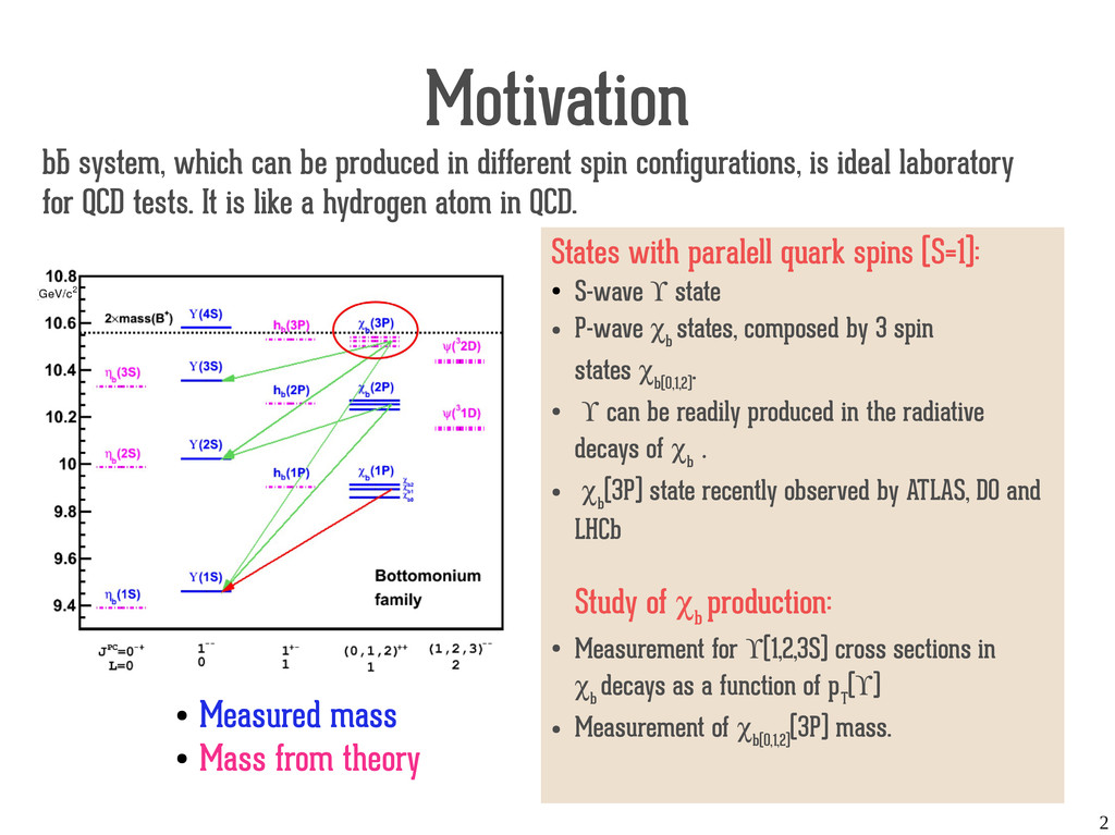
2. 2 Motivation bb system, which can be produced in different spin configurations, is ideal laboratory ̄ for QCD tests. It is like a hydrogen atom in QCD. States with paralell quark spins (S=1): • S-wave ϒ state • P-wave χ b states, composed by 3 spin states χ b(0,1,2) . • ϒ can be readily produced in the radiative decays of χ b . • χ b (3P) state recently observed by ATLAS, D0 and LHCb Study of χ b production: • Measurement for ϒ(1,2,3S) cross sections in χ b decays as a function of p T (ϒ) • Measurement of χ b(0,1,2) (3P) mass. • Measured mass • Mass from theory
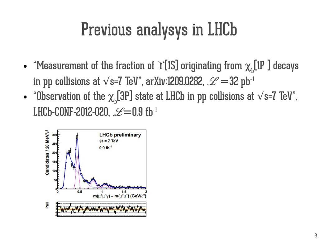
3. 3 Previous analysys in LHCb • “Measurement of the fraction of ϒ(1S) originating from χ b (1P ) decays in pp collisions at s=7 TeV”, arXiv:1209.0282, √ L =32 pb−1 • “Observation of the χ b (3P) state at LHCb in pp collisions at s=7 TeV”, √ LHCb-CONF-2012-020, L=0.9 fb−1
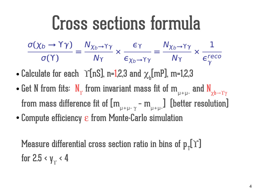
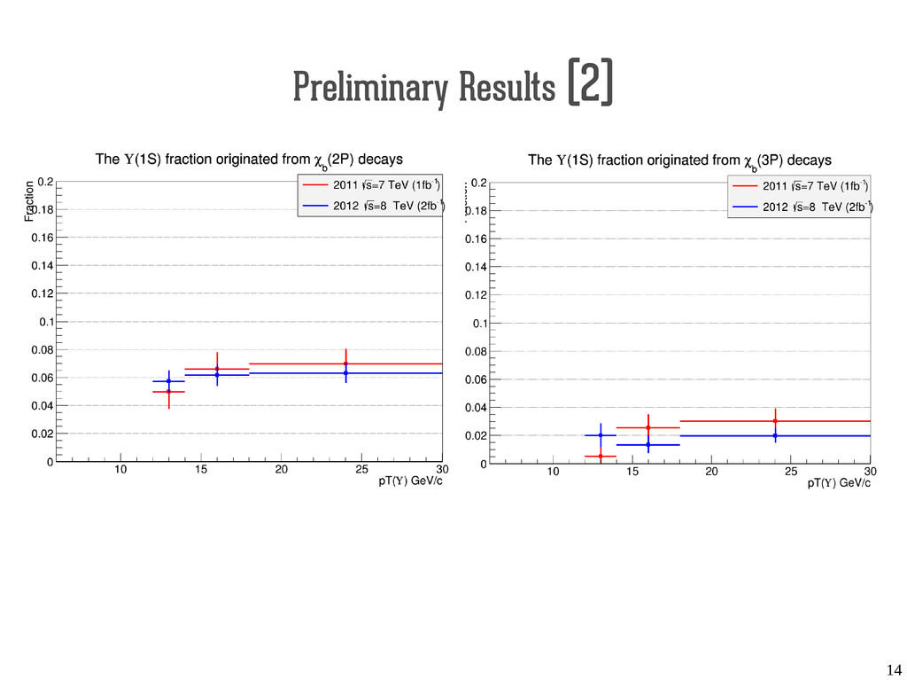
4. 4 Cross sections formula • Calculate for each ϒ(nS), n=1,2,3 and χ b (mP), m=1,2,3 • Get N from fits: N ϒ from invariant mass fit of m µ+µ- and N χb→ϒγ from mass difference fit of [m µ+µ- γ – m µ+µ- ] (better resolution) • Compute efficiency ε from Monte-Carlo simulation Measure differential cross section ratio in bins of p T (ϒ) for 2.5 < y ϒ < 4
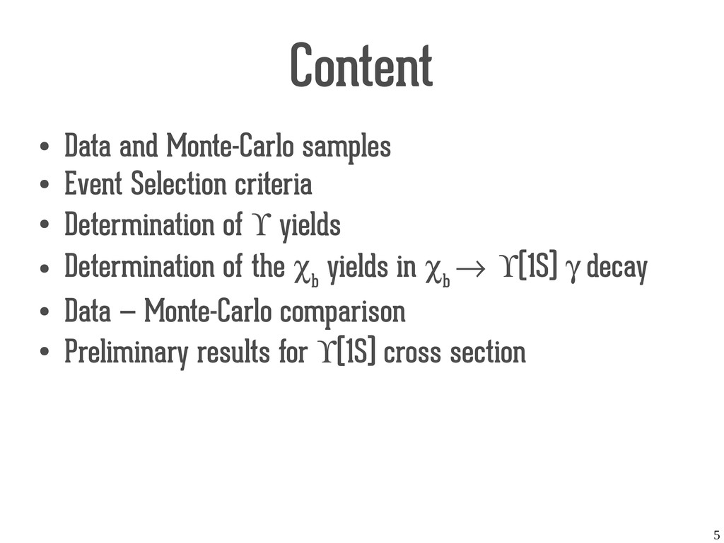
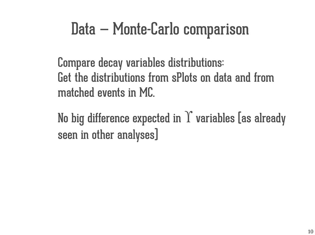
5. 5 Content • Data and Monte-Carlo samples • Event Selection criteria • Determination of ϒ yields • Determination of the χ b yields in χ b → ϒ(1S) γ decay • Data — Monte-Carlo comparison • Preliminary results for ϒ(1S) cross section
6. 6 Data and Monte-Carlo samples • √s=7 TeV: Reco14, Stripping 20r1, WGBandQSelection3, BOTTOM.MDST. L=1089 pb-1 • √s=8 TeV: Reco14, Stripping 20, WGBandQSelection3, BOTTOM.MDST. L=2011 pb-1 • Monte Carlo: MC11a, Reco12a, inclusive χ b0,1,2 (1,2,3P) decays. 5E+5 events for each χ b state and magnet direction. — χ b0,1,2 (2,3P) could not be generated directly, so they are defined as χ b1,2 (1P), but with redefined mass and decay channels.
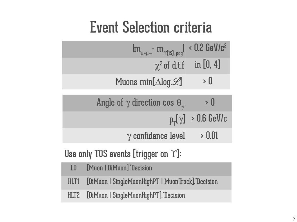
7. 7 Event Selection criteria |m µ+µ− - m ϒ(1S), pdg | < 0.2 GeV/c2 χ2 of d.t.f in [0, 4] Muons min(∆logL] > 0 Angle of γ direction cos θ γ > 0 p T (γ] > 0.6 GeV/c γ confidence level > 0.01 Use only TOS events (trigger on ϒ]: L0 (Muon | DiMuon).*Decision HLT1 (DiMuon | SingleMuonHighPT | MuonTrack).*Decision HLT2 (DiMuon | SingleMuonHighPT).*Decision
8. 8 Determination of ϒ yields ϒ(1S) ϒ(2S) ϒ(3S) Y(1S) signal: f*CB Y(1S)(1) (µ Y(1S) , σ Y(1S) , α, n] + (1-f)CB Y(1S)(2) (µ Y(1S) , σ Y(1S) , -α, n] Y(2S) signal: CB Y(2S) (µ Y(2S) , σ Y(2S) , α, n] Y(3S) signal: CB Y(3S) (µ Y(3S) , σ Y(3S) , α, n] • Floating parameters: f, µ Y(1,2,3S) , σ Y(1S) , τ, a 1 • Constant parameters: α, n • Constraints: σ Y(2S) = σ Y(1S) * (µ Y(2S) /µ Y(1S) ], σ Y(3S) = σ Y(1S) * (µ Y(3S) /µ Y(1S) ] Signal: the sum of Crystal Ball functions, one for each of the Y(2S), Y(3S) and two for Y(1S). Background: e-τx *(a 1 x) √s=8 TeV p T (ϒ) > 6 GeV/c 6.5e+5 2e+5 1.1e+5 α 1.28 n 4 B 1314200 ± 1500 N1S 651760 ± 969 f 0.749 ± 0.001 N2S 197750 ± 597 N3S 112670 ± 482 dm2s 0.56421 ± 0.00018 dm3s 0.89588 ± 0.00024 µ Y(1S) 9.4677 ± 0.00076 a 1 0.1098 ± 0.0092 σ Y(1S) 0.045809 ± 0.000065 τ -0.548 ± 0.011
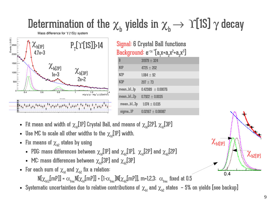
9. 9 Determination of the χ b yields in χ b → ϒ(1S) γ decay χ b(1P) Signal: 6 Crystal Ball functions Background: e-τx *(a 1 x+a 2 x2+a 3 x3) • Fit mean and width of χ b1 (1P) Crystal Ball, and means of χ b1 (2P), χ b1 (3P) • Use MC to scale all other widths to the χ b1 (1P) width. • Fix means of χ b2 states by using • PDG: mass differences between χ b1 (1P) and χ b2 (1P), χ b1 (2P) and χ b2 (2P) • MC: mass differences between χ b1 (3P) and χ b2 (3P) • For each sum of χ b1 and χ b2 fix a relation: N[χ b1,2 (mP)] = α frac N[χ b1 (mP)] + (1-α frac )N[χ b2 (mP)], m=1,2,3; α frac fixed at 0.5 • Systematic uncertainties due to relative contributions of χ b1 and χ b2 states ~ 5% on yields (see backup] P T (ϒ(1S)]>14 χ b(2P) χ b(3P) χ b1(1P) χ b2(1P) 4.7e+3 1e+3 2e+2 B 31979 ± 324 N1P 4725 ± 202 N2P 1.084 ± 92 N3P 207 ± 73 mean_b1_1p 0.42989 ± 0.00076 mean_b1_2p 0.7922 ± 0.0035 mean_b1_3p 1.074 ± 0.035 sigma_1P 0.02167 ± 0.00087
10. 10 Data — Monte-Carlo comparison Compare decay variables distributions: Get the distributions from sPlots on data and from matched events in MC. No big difference expected in ϒ variables (as already seen in other analyses)
11. 11 p T (ϒ) χ b (1P) χ b (2P) χ b (3P) p T (ϒ) p T (ϒ) p T (χ b (1P)) p T (χ b (2P)) p T (χ b (3P)) — Monte-Carlo — Data
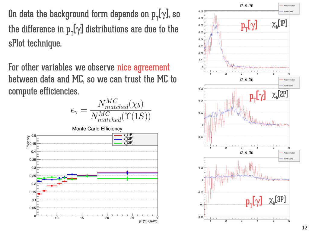
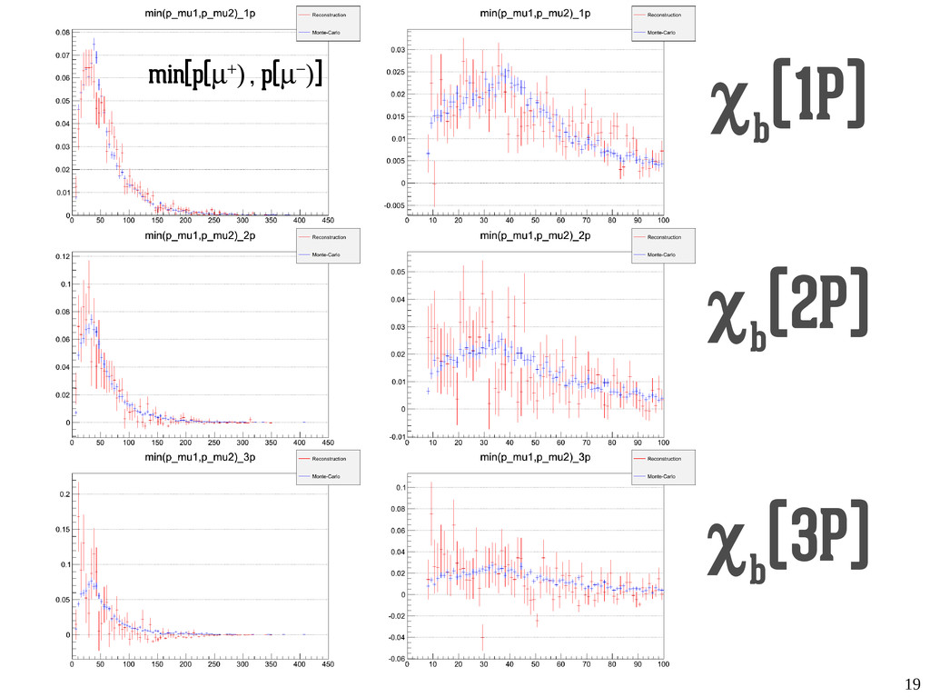
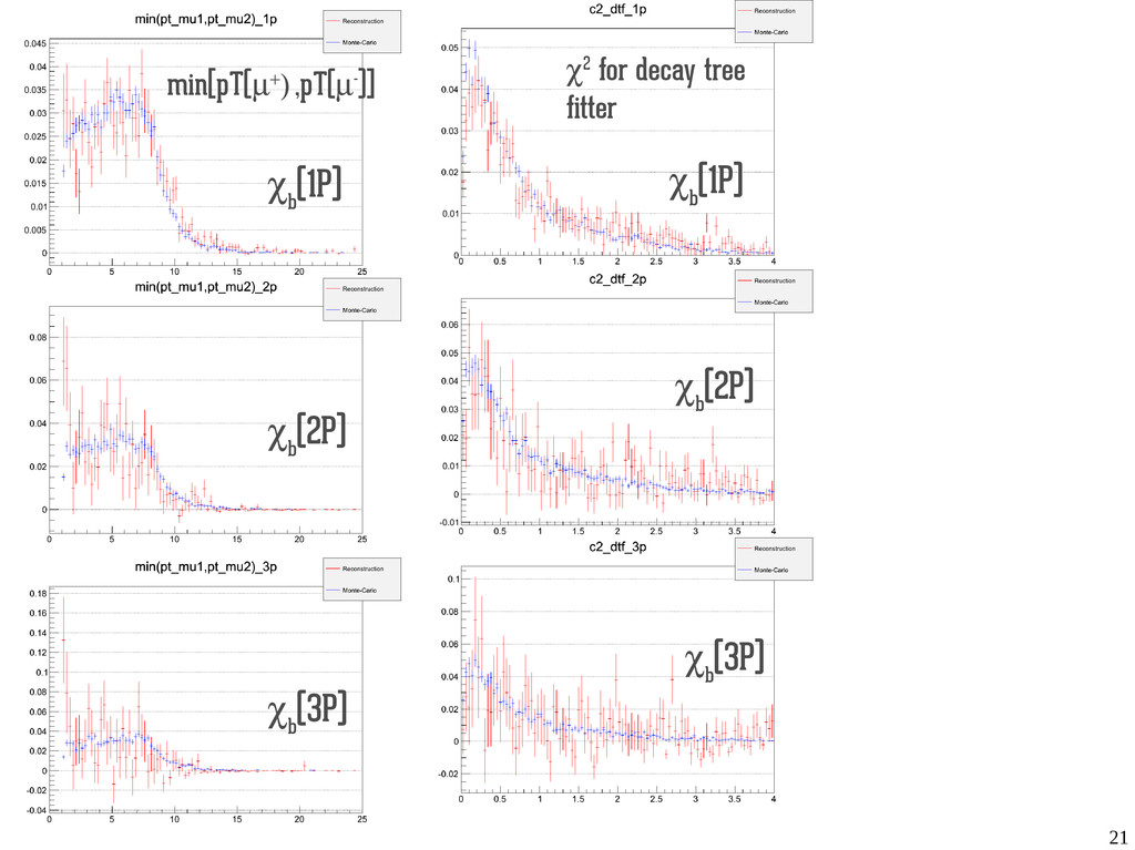
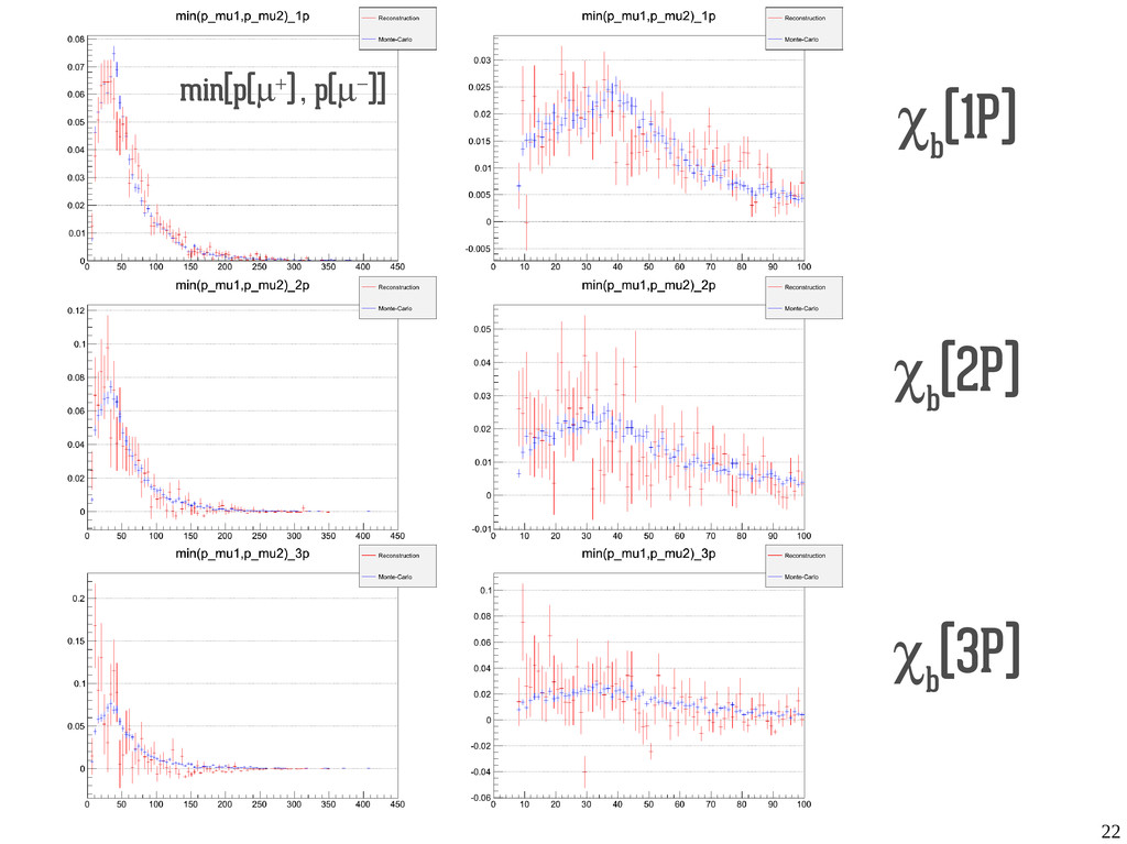
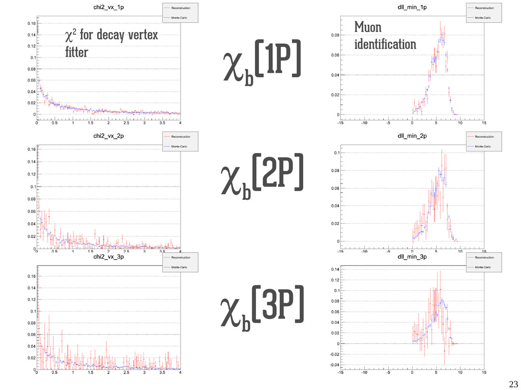
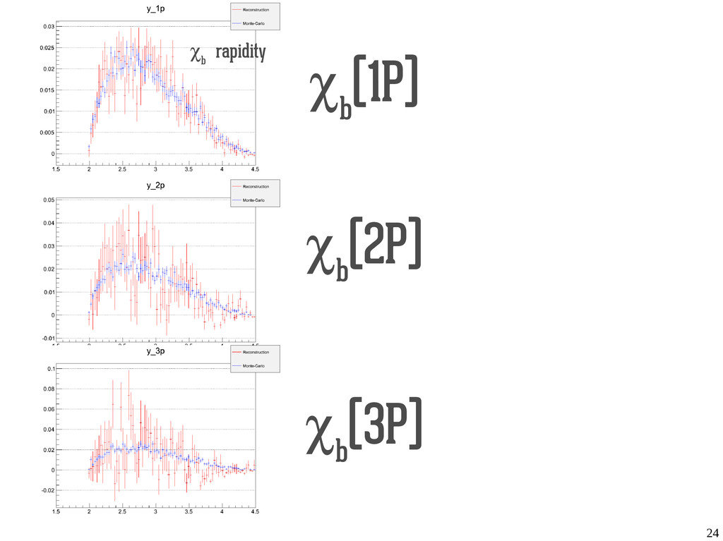
12. 12 p T (γ) χ b (1P) p T (γ) p T (γ) χ b (2P) χ b (3P) On data the background form depends on p T (γ], so the difference in p T (γ] distributions are due to the sPlot technique. For other variables we observe nice agreement between data and MC, so we can trust the MC to compute efficiencies.
13. 13 Preliminary Results (1)
14. 14 Preliminary Results (2)
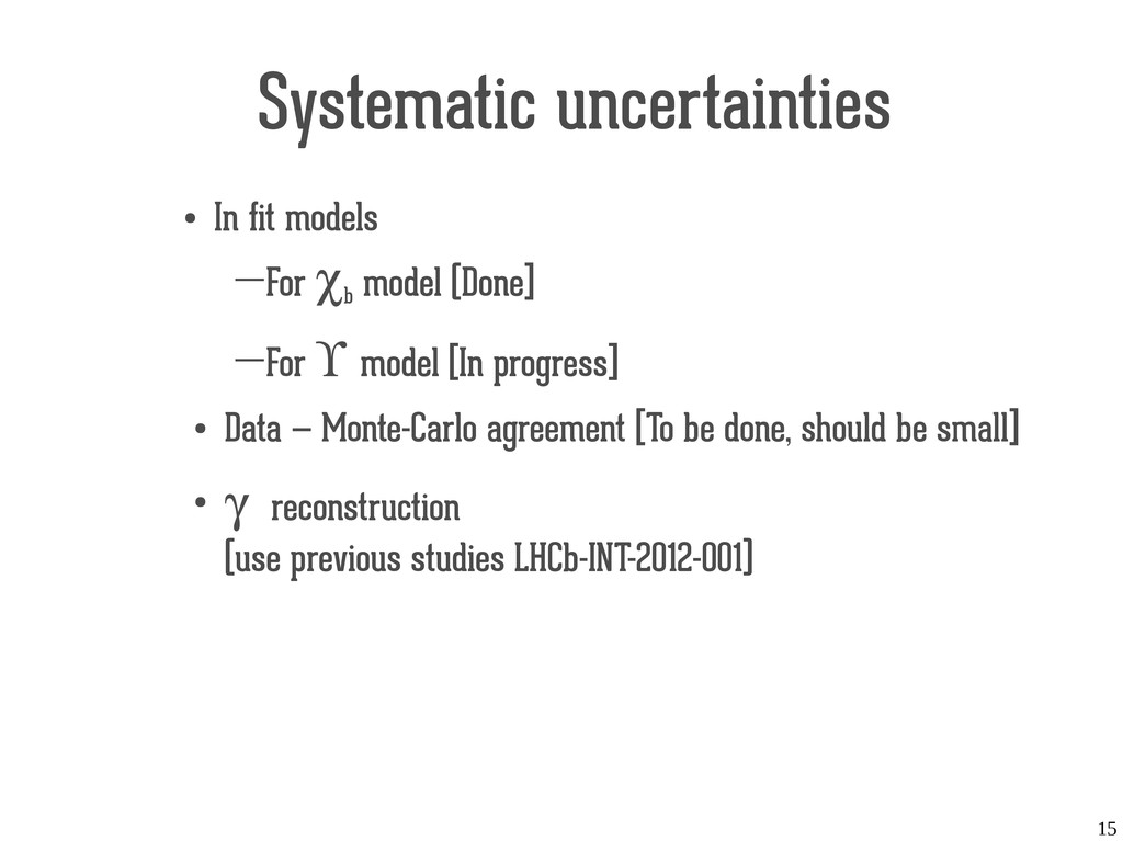
15. 15 Systematic uncertainties • In fit models ―For χb model (Done] ―For ϒ model [In progress] • Data — Monte-Carlo agreement [To be done, should be small] • γ reconstruction (use previous studies LHCb-INT-2012-001)
16. 16 ToDo • Finalize systematic uncertainties • Documentation • Study of ϒ(2,3S) fractions • Measurement for rapidity bins • Precise measurement of χb (3P) mass
17. 17 Backup
18. 18 Systematic uncertainties Constraint N[χ b (1P)] change(%) N[χ b (2P)] change(%) N[χ b (3P)] change(%) N[χ b (2P)]/N[χ b (1P)] change(%) N[χ b (3P)]/N[χ b (1P)] change(%) α frac [χ b (1P)] = 0 3 3 3 0 1 α frac [χ b (1P)] = 1 3 3 3 0 1 α frac [χ b (2P)] = 0 2 -2 1 -4 0 α frac [χ b (2P)] = 1 0 -1 0 -1 0 α frac [χ b (3P)] = 0 0 0 -1 0 -1 α frac [χ b (3P)] = 1 0 0 0 0 0 Fix max PDG mass diff between χ b1 (1P) and χ b2 (1P) 2 -4 7 -6 -8 Fix max PDG mass diff between χ b1 (2P) and χ b2 (2P) 0 0 0 0 0 • Systematic uncertainties due to relative contributions of χ b1 and χ b2 states • Other systematic uncertainties are under study.
19. 19 χ b (1P) χ b (2P) χ b (3P) min[p(µ+) , p(µ−)]
20. 20 Data — Monte-Carlo comparison
21. 21 χ b (1P) χ b (2P) χ b (3P) min[pT(µ+) ,pT(µ-)] χ2 for decay tree fitter χ b (1P) χ b (2P) χ b (3P)
22. 22 χ b (1P) χ b (2P) χ b (3P) min[p(µ+) , p(µ−)]
23. 23 χ b (1P) χ b (2P) χ b (3P) Muon identification χ2 for decay vertex fitter
24. 24 χ b (1P) χ b (2P) χ b (3P) χ b rapidity