Ph.D final exam

Transcript

1. High Level Trigger software performance profiling and χb production study at the LHCb experiment Alexander Mazurov Tutor: Concezio Bozzi University of Ferrara (Italy) & CERN 7 March 2014 1/46
2. Plan 1 LHCb experiment 2 Measuring Υ(NS) (N=1, 2, 3) fraction originating from χb decays and χb(3P) mass: Motivation Datasets Determination of Υ yields Determination of χb yields in the following decays: χb (1, 2, 3P) → Υ(1S)γ χb (2, 3P) → Υ(2S)γ χb (3P) → Υ(3S)γ Monte-Carlo efficiencies Systematic uncertainties Results 3 Summary 4 Backup: HLT profiler 2/46
3. The LHC Accelerator System The main LHC design parameters: Circumference 27 km Center-of-mass energy 14 TeV Injection energy 450 GeV Field at 2 × 450 GeV 0.535 T Field at 2 × 7 TeV 8 T Helium temperature 2K Luminosity 1034 cm−2s−1 Bunch spacing 25 ns Luminosity lifetime 10 hr Time between 2 fills 7 hr The LHC operated mainly at center-of-mass energies of 7 TeV and 8 TeV in 2011 and 2012, respectively. In 2015, after the long shutdown, LHC is planned to reach energy of 13 TeV. 3/46
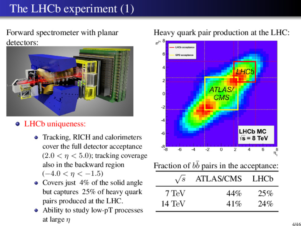
4. The LHCb experiment (1) Forward spectrometer with planar detectors: LHCb uniqueness: Tracking, RICH and calorimeters cover the full detector acceptance (2.0 < η < 5.0); tracking coverage also in the backward region (−4.0 < η < −1.5) Covers just 4% of the solid angle but captures 25% of heavy quark pairs produced at the LHC. Ability to study low-pT processes at large η Heavy quark pair production at the LHC: Fraction of b¯ b pairs in the acceptance: √ s ATLAS/CMS LHCb 7 TeV 44% 25% 14 TeV 41% 24% 4/46
5. The LHCb experiment (2) Excellent tracking performance High quality particle identification: robust hadron ID + photon/lepton/hadron separation Selective and flexible trigger system 5/46
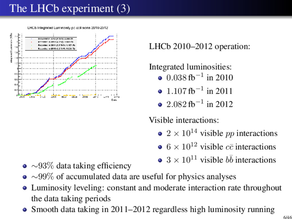
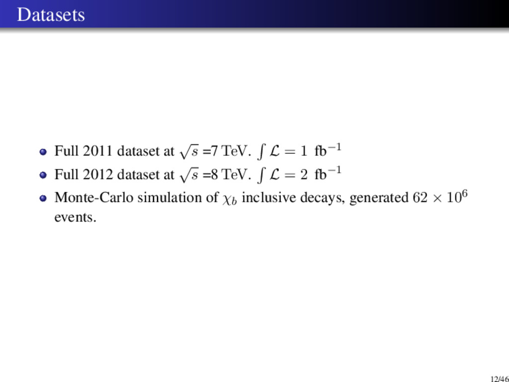
6. The LHCb experiment (3) LHCb 2010–2012 operation: Integrated luminosities: 0.038 fb−1 in 2010 1.107 fb−1 in 2011 2.082 fb−1 in 2012 Visible interactions: 2 × 1014 visible pp interactions 6 × 1012 visible c¯ c interactions 3 × 1011 visible b¯ b interactions ∼93% data taking efficiency ∼99% of accumulated data are useful for physics analyses Luminosity leveling: constant and moderate interaction rate throughout the data taking periods Smooth data taking in 2011–2012 regardless high luminosity running 6/46
7. Study of χb production 7/46
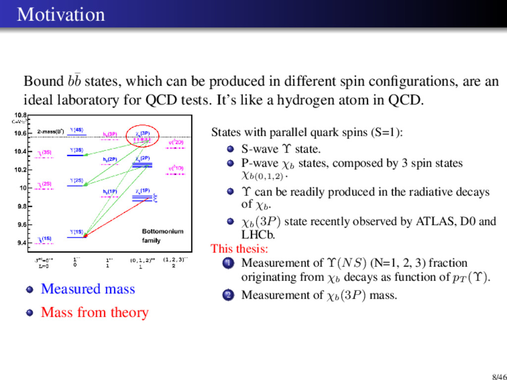
8. Motivation Bound b¯ b states, which can be produced in different spin configurations, are an ideal laboratory for QCD tests. It’s like a hydrogen atom in QCD. Measured mass Mass from theory States with parallel quark spins (S=1): S-wave Υ state. P-wave χb states, composed by 3 spin states χb(0,1,2) . Υ can be readily produced in the radiative decays of χb. χb (3P) state recently observed by ATLAS, D0 and LHCb. This thesis: 1 Measurement of Υ(NS) (N=1, 2, 3) fraction originating from χb decays as function of pT (Υ). 2 Measurement of χb (3P) mass. 8/46
9. Previous analysis at LHCb ”Measurement of the fraction of Υ(1S) originating from χb(1P) in pp collisions at √ s =7 TeV ”, arXiv:1209.0282, L = 32 pb−1 ”Observation of the χb(3P) state at LHCb in pp collisions at √ s =7 TeV ”, LHCb-CONF-2012-020, L = 0.9 fb−1. 9/46
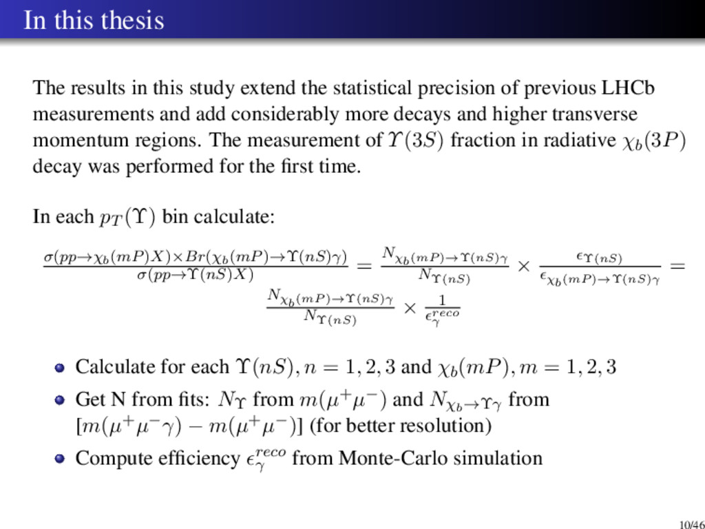
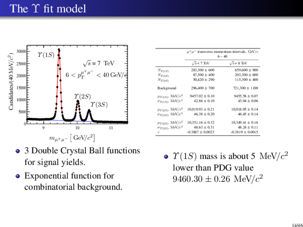
10. In this thesis The results in this study extend the statistical precision of previous LHCb measurements and add considerably more decays and higher transverse momentum regions. The measurement of Υ(3S) fraction in radiative χb(3P) decay was performed for the first time. In each pT (Υ) bin calculate: σ(pp→χb(mP)X)×Br(χb(mP)→Υ(nS)γ) σ(pp→Υ(nS)X) = Nχb(mP )→Υ(nS)γ NΥ(nS) × Υ(nS) χb(mP )→Υ(nS)γ = Nχb(mP )→Υ(nS)γ NΥ(nS) × 1 reco γ Calculate for each Υ(nS), n = 1, 2, 3 and χb(mP), m = 1, 2, 3 Get N from fits: NΥ from m(µ+µ−) and Nχb→Υγ from [m(µ+µ−γ) − m(µ+µ−)] (for better resolution) Compute efficiency reco γ from Monte-Carlo simulation 10/46
11. Analysis Plan 1 Datasets 2 Determination of Υ yields 3 Determination of χb yields in the following decays: χb (1, 2, 3P) → Υ(1S)γ χb (2, 3P) → Υ(2S)γ χb (3P) → Υ(3S)γ 4 Monte-Carlo efficiencies 5 Systematic uncertainties 6 Results 11/46
12. Datasets Full 2011 dataset at √ s =7 TeV. L = 1 fb−1 Full 2012 dataset at √ s =8 TeV. L = 2 fb−1 Monte-Carlo simulation of χb inclusive decays, generated 62 × 106 events. 12/46
13. The Υ selection Description Requirement Υ rapidity1 2.0 < yΥ < 4.5 Track fit quality χ2/ndf < 4 Track pT > 1 GeV/c Primary vertex probability > 0.5% Luminous region |zPV | < 0.5m and x2 PV + y2 PV < 100mm2 Kullback-Leibler distance > 5000 Muon and hadron hypotheses ∆ log Lµ−h > 0 Muon probability ProbNN > 0.5 Trigger lines: L0 L0DiMuon HLT1 Hlt1DiMuonHighMass HLT2 HLT2DiMuonB 1y = 1 2 ln(E+pL E−pL ), where pL is the component of the momentum along the beam axis 13/46
14. The Υ fit model 9 10 11 0 5000 10000 15000 20000 25000 30000 Candidates/(40 MeV/c2) mµ+µ− GeV/c2 √ s = 7 TeV 6 < pµ+µ− T < 40 GeV/c Υ(1S) Υ(2S) Υ(3S) 3 Double Crystal Ball functions for signal yields. Exponential function for combinatorial background. µ+µ− transverse momentum intervals, GeV/c 6 – 40 √ s = 7 TeV √ s = 8 TeV NΥ(1S) 283,300 ± 600 659,600 ± 900 NΥ(2S) 87,500 ± 400 203,300 ± 600 NΥ(3S) 50,420 ± 290 115,300 ± 400 Background 296,400 ± 700 721,300 ± 1100 µΥ(1S) , MeV/c2 9457.02 ± 0.10 9455.58 ± 0.07 σΥ(1S) , MeV/c2 42.86 ± 0.10 43.04 ± 0.06 µΥ(2S) , MeV/c2 10,019.03 ± 0.21 10,018.05 ± 0.14 σΥ(2S) , MeV/c2 46.38 ± 0.20 46.45 ± 0.14 µΥ(3S) , MeV/c2 10,351.16 ± 0.32 10,349.41 ± 0.16 σΥ(3S) , MeV/c2 48.63 ± 0.31 48.24 ± 0.11 τ -0.3887 ± 0.0023 -0.3819 ± 0.0015 Υ(1S) mass is about 5 MeV/c2 lower than PDG value 9460.30 ± 0.26 MeV/c2 14/46
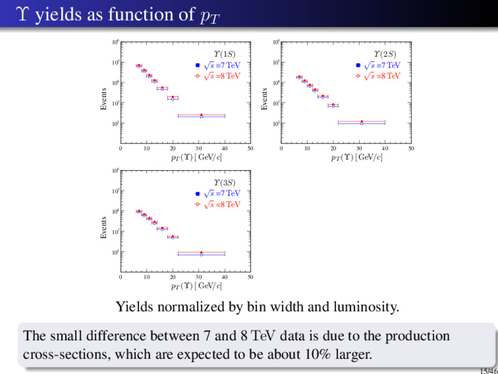
15. Υ yields as function of pT 0 10 20 30 40 50 2 10 3 10 4 10 5 10 6 10 0 10 20 30 40 50 2 10 3 10 4 10 5 10 6 10 0 10 20 30 40 50 2 10 3 10 4 10 5 10 6 10 Events pT (Υ) [ GeV/c] Υ(3S) Events pT (Υ) [ GeV/c] Υ(1S) Events pT (Υ) [ GeV/c] Υ(2S) √ s =7 TeV √ s =8 TeV √ s =7 TeV √ s =8 TeV √ s =7 TeV √ s =8 TeV Yields normalized by bin width and luminosity. The small difference between 7 and 8 TeV data is due to the production cross-sections, which are expected to be about 10% larger. 15/46
16. χb selection In this study photons reconstructed using the calorimeter information. Another approach uses photon conversions in e+e− pairs — this method has better invariant mass resolution, but requires more statistics. Cuts on γ: Transverse momentum of γ pT (γ) > 600 MeV/c Polar angle of γ in the µ+µ−γ rest frame cos θγ > 0 Confidence level of γ cl(γ) > 0.01 Dimuon mass windows: Decay Cut Description χb(1, 2, 3P) → Υ(1S) 9310 < µ+µ− < 9600 MeV/c 3σΥ(1S) < µ+µ− < 2.5σΥ(1S) MeV/c χb(2, 3P) → Υ(2S) 9870 < µ+µ− < 10090 MeV/c 3σΥ(2S) < µ+µ− < σΥ(2S) MeV/c χb(3P) → Υ(3S) 10300 < µ+µ− < 10526 MeV/c σΥ(3S) < µ+µ− < 3σΥ(3S) MeV/c 16/46
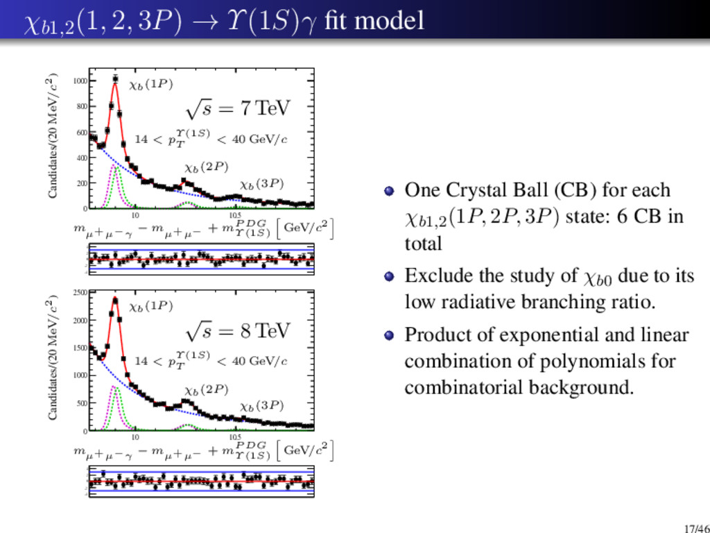
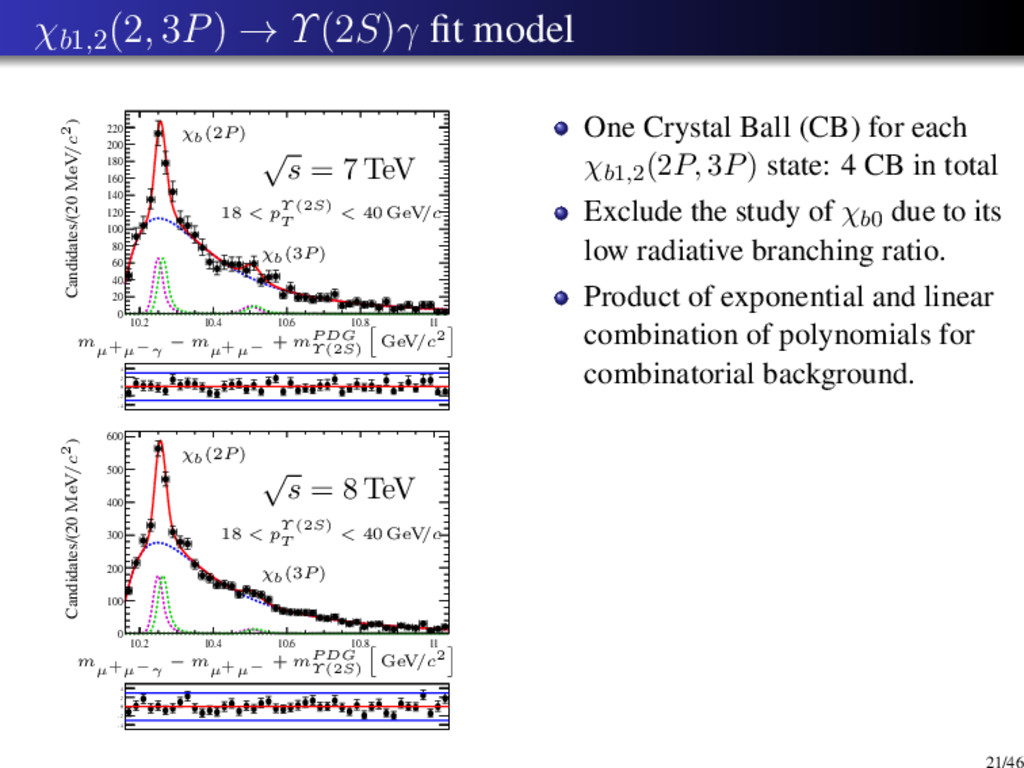
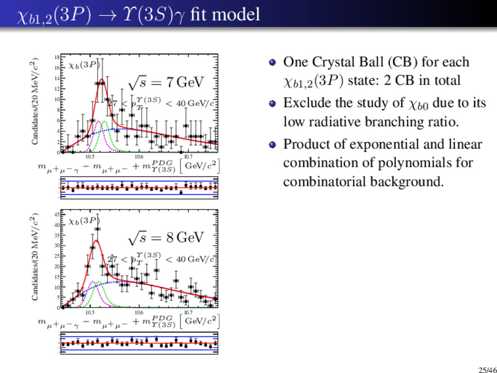
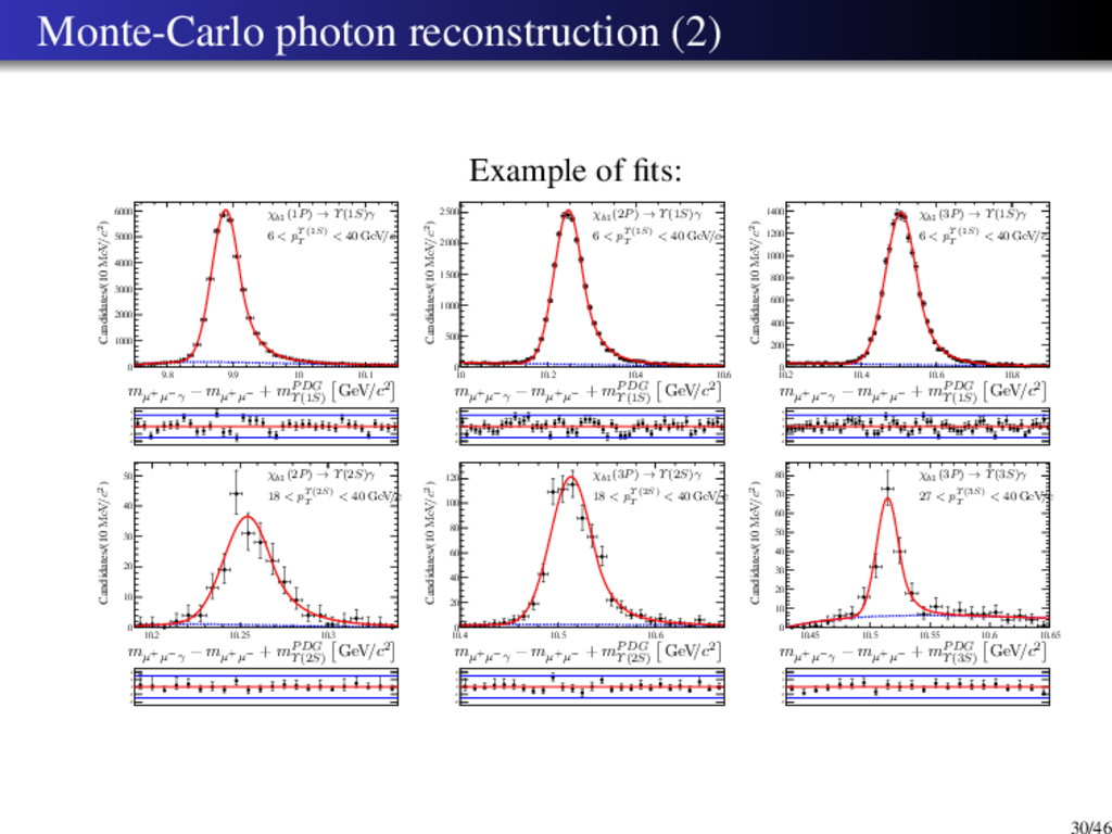
17. χb1,2 (1, 2, 3P) → Υ(1S)γ fit model 10 10.5 0 500 1000 1500 2000 2500 -4 -2 0 2 4 10 10.5 0 200 400 600 800 1000 -4 -2 0 2 4 Candidates/(20 MeV/c2) m µ+µ−γ − m µ+µ− + mP DG Υ (1S) GeV/c2 √ s = 8 TeV 14 < pΥ (1S) T < 40 GeV/c Candidates/(20 MeV/c2) m µ+µ−γ − m µ+µ− + mP DG Υ (1S) GeV/c2 √ s = 7 TeV 14 < pΥ (1S) T < 40 GeV/c χb(1P ) χb(2P ) χb(3P ) χb(1P ) χb(2P ) χb(3P ) One Crystal Ball (CB) for each χb1,2(1P, 2P, 3P) state: 6 CB in total Exclude the study of χb0 due to its low radiative branching ratio. Product of exponential and linear combination of polynomials for combinatorial background. 17/46
18. χb1,2 (1, 2, 3P) → Υ(1S)γ fit model (2) Free parameters: µχb1(1P), yields and background parameters. Linked parameters for χb1 and χb2 signals: µχb2(jP ) = µχb1(jP ) + ∆mP DG χb2(jP ) , j=1,2 µχb2(3P ) = µχb1(3P ) + ∆mtheory χb2(3P ) Nχb = λNχb1 + (1 − λ)Nχb2 σχb2 = σχb1 Other linked parameters: µχb1(2P ) = µχb1(1P ) + ∆mP DG χb1(2P ) µχb1(3P ) = µχb1(1P ) + ∆mχb1(3P ) (∆mχb1(3P ) measured in this study) Fixed parameters from MC study: σχb1(1P ) scaled by 1.17, σχb1(2P ) σχb1(1P ) , σχb1(3P ) σχb1(1P ) α and n parameters of CB. Υ(1S) transverse momentum intervals, GeV/c 14 – 40 √ s = 7 TeV √ s = 8 TeV Nχb(1P) 2090 ± 80 5070 ± 130 Nχb(2P) 450 ± 50 1010 ± 80 Nχb(3P) 150 ± 40 220 ± 60 Background 8830 ± 130 23,910 ± 210 µχb1(1P) , MeV/c2 9889.7 ± 1.0 9890.3 ± 0.7 σχb1(1P) , MeV/c2 22.0 22.5 σχb1(2P) /σχb1(1P) 1.5 1.5 σχb1(3P) /σχb1(1P) 1.86 1.86 τ -2.6 ± 0.5 -3.27 ± 0.30 c0 -0.08 ± 0.12 0.07 ± 0.06 c1 1.33 ± 0.04 0.29 ± 0.04 χ2/n.d.f 1.03 1.24 χb1(1P ) mass agrees with the PDG value 9892.78 ± 0.26 (stat) ± 0.31 (syst) MeV/c2. 18/46
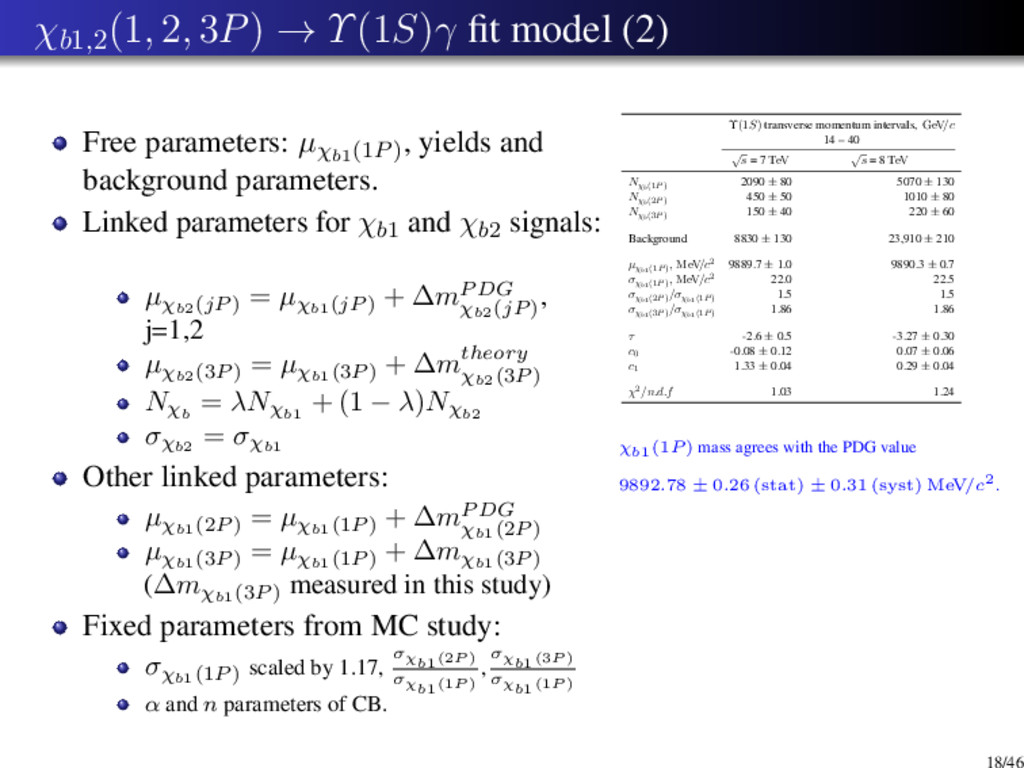
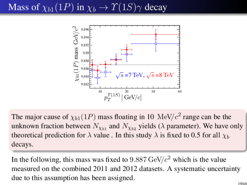
19. Mass of χb1 (1P) in χb → Υ(1S)γ decay 10 20 30 40 9.882 9.884 9.886 9.888 9.89 9.892 9.894 9.896 √ s =7 TeV, √ s =8 TeV χb1(1P) mass GeV/c2 pΥ(1S) T [ GeV/c] The major cause of χb1(1P) mass floating in 10 MeV/c2 range can be the unknown fraction between Nχb1 and Nχb2 yields (λ parameter). We have only theoretical prediction for λ value . In this study λ is fixed to 0.5 for all χb decays. In the following, this mass was fixed to 9.887 GeV/c2 which is the value measured on the combined 2011 and 2012 datasets. A systematic uncertainty due to this assumption has been assigned. 19/46
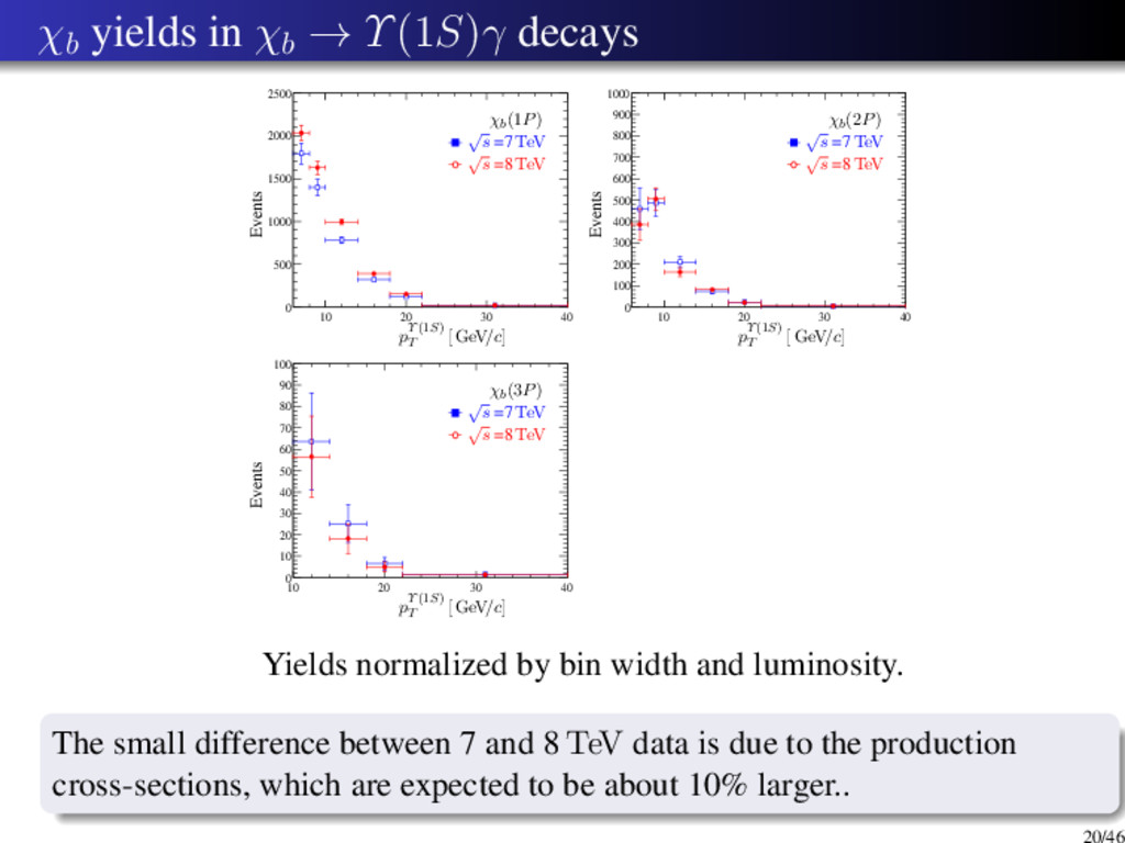
20. χb yields in χb → Υ(1S)γ decays 10 20 30 40 0 10 20 30 40 50 60 70 80 90 100 10 20 30 40 0 500 1000 1500 2000 2500 10 20 30 40 0 100 200 300 400 500 600 700 800 900 1000 Events pΥ(1S) T [ GeV/c] χb(3P) Events pΥ(1S) T [ GeV/c] χb(1P) Events pΥ(1S) T [ GeV/c] χb(2P) √ s =7 TeV √ s =8 TeV √ s =7 TeV √ s =8 TeV √ s =7 TeV √ s =8 TeV Yields normalized by bin width and luminosity. The small difference between 7 and 8 TeV data is due to the production cross-sections, which are expected to be about 10% larger.. 20/46
21. χb1,2 (2, 3P) → Υ(2S)γ fit model 10.2 10.4 10.6 10.8 11 0 100 200 300 400 500 600 -4 -2 0 2 4 10.2 10.4 10.6 10.8 11 0 20 40 60 80 100 120 140 160 180 200 220 -4 -2 0 2 4 Candidates/(20 MeV/c2) m µ+µ−γ − m µ+µ− + mP DG Υ (2S) GeV/c2 √ s = 8 TeV 18 < pΥ (2S) T < 40 GeV/c Candidates/(20 MeV/c2) m µ+µ−γ − m µ+µ− + mP DG Υ (2S) GeV/c2 √ s = 7 TeV 18 < pΥ (2S) T < 40 GeV/c χb(2P ) χb(3P ) χb(2P ) χb(3P ) One Crystal Ball (CB) for each χb1,2(2P, 3P) state: 4 CB in total Exclude the study of χb0 due to its low radiative branching ratio. Product of exponential and linear combination of polynomials for combinatorial background. 21/46
22. χb1,2 (2, 3P) → Υ(2S)γ fit model (2) Free parameters: µχb1(2P), yields and background parameters. Linked parameters for χb1 and χb2 signals: µχb2(2P ) = µχb1(2P ) + ∆mP DG χb2(2P ) µχb2(3P ) = µχb1(3P ) + ∆mtheory χb2(3P ) Nχb = λNχb1 + (1 − λ)Nχb2 σχb2 = σχb1 Other linked parameters: µχb1(3P ) = µχb1(1P ) + ∆mχb1(3P ) (∆mχb1(3P ) measured in this study) Fixed parameters from MC study: σχb1(2P ) , σχb1(3P ) σχb1(2P ) α and n parameters of CB. Υ(2S) transverse momentum intervals, GeV/c 18 – 40 √ s = 7 TeV √ s = 8 TeV Nχb(2P) 237 ± 29 650 ± 50 Nχb(3P) 50 ± 17 78 ± 26 Background 1830 ± 50 4600 ± 80 µχb1(2P) , MeV/c2 10,249.1 ± 2.2 10,249.9 ± 1.3 σχb1(2P) , MeV/c2 13.0 13.3 σχb1(3P) /σχb1(2P) 1.65 1.65 τ -7.5 ± 0.8 -7.7 ± 0.5 c0 0.431 ± 0.027 0.435 ± 0.016 c1 -2.07 ± 0.09 -2.12 ± 0.05 c2 0.79 ± 0.36 0.79 ± 0.17 χ2/n.d.f 0.98 1.35 The mass of χb1(2P ) is about 6 MeV/c2 less than value in PDG (10.25546 GeV/c2). 22/46
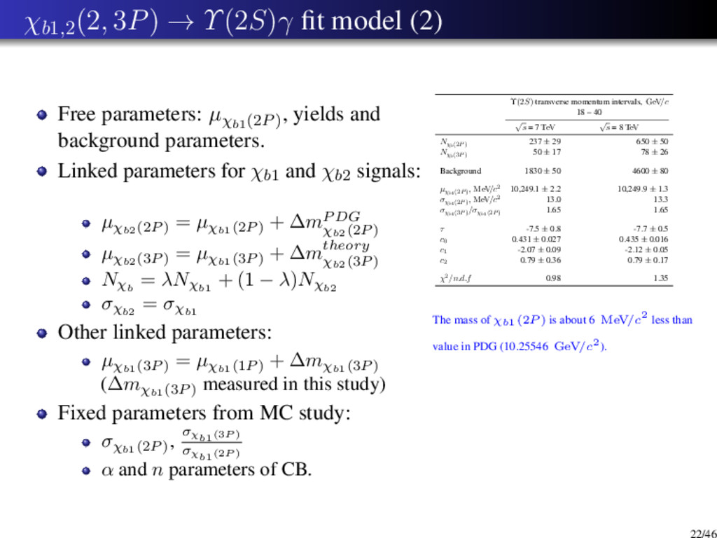
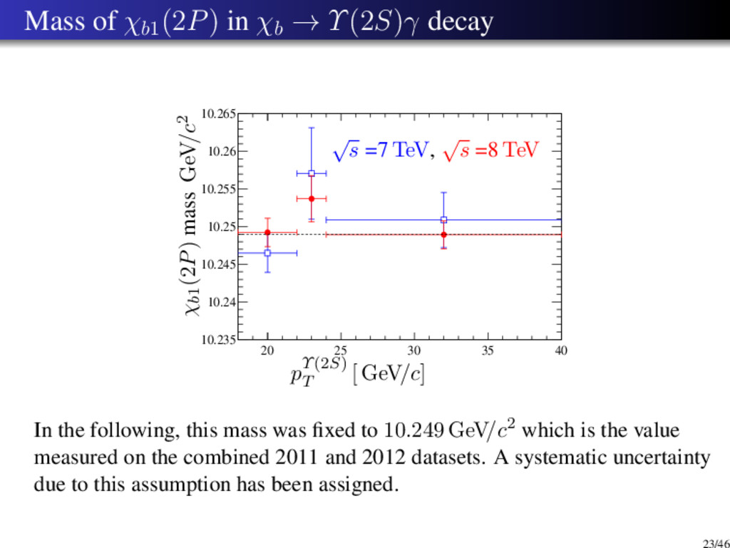
23. Mass of χb1 (2P) in χb → Υ(2S)γ decay 20 25 30 35 40 10.235 10.24 10.245 10.25 10.255 10.26 10.265 √ s =7 TeV, √ s =8 TeV χb1(2P) mass GeV/c2 pΥ(2S) T [ GeV/c] In the following, this mass was fixed to 10.249 GeV/c2 which is the value measured on the combined 2011 and 2012 datasets. A systematic uncertainty due to this assumption has been assigned. 23/46
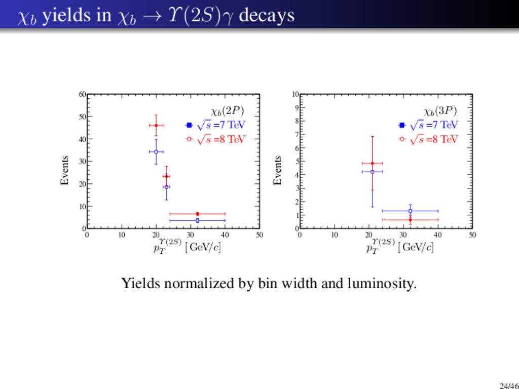
24. χb yields in χb → Υ(2S)γ decays 0 10 20 30 40 50 0 10 20 30 40 50 60 0 10 20 30 40 50 0 1 2 3 4 5 6 7 8 9 10 Events pΥ(2S) T [ GeV/c] χb(2P) Events pΥ(2S) T [ GeV/c] χb(3P) √ s =7 TeV √ s =8 TeV √ s =7 TeV √ s =8 TeV Yields normalized by bin width and luminosity. 24/46
25. χb1,2 (3P) → Υ(3S)γ fit model 10.5 10.6 10.7 0 5 10 15 20 25 30 35 40 45 -4 -2 0 2 4 10.5 10.6 10.7 0 2 4 6 8 10 12 14 16 18 -4 -2 0 2 4 Candidates/(20 MeV/c2) m µ+µ−γ − m µ+µ− + mP DG Υ (3S) GeV/c2 √ s = 8 GeV 27 < pΥ (3S) T < 40 GeV/c Candidates/(20 MeV/c2) m µ+µ−γ − m µ+µ− + mP DG Υ (3S) GeV/c2 √ s = 7 GeV 27 < pΥ (3S) T < 40 GeV/c χb(3P ) χb(3P ) One Crystal Ball (CB) for each χb1,2(3P) state: 2 CB in total Exclude the study of χb0 due to its low radiative branching ratio. Product of exponential and linear combination of polynomials for combinatorial background. 25/46
26. χb1,2 (3P) → Υ(3S)γ fit model (2) Free parameters: µχb1(3P), σχb1(3P), yields, background parameters. Linked parameters for χb1 and χb2 signals: µχb2(3P ) = µχb1(3P ) + ∆mtheory χb2(3P ) Nχb = λNχb1 + (1 − λ)Nχb2 σχb2 = σχb1 Fixed parameters from MC study: α and n parameters of CB. Υ(3S) transverse momentum intervals, GeV/c 27 – 40 √ s = 7 TeV √ s = 8 TeV Nχb(3P) 31 ± 12 72 ± 16 Background 97 ± 14 283 ± 21 µχb1(3P) , MeV/c2 10,517 ± 4 10,504.0 ± 2.5 σχb1(3P) , MeV/c2 9 ± 6 8.3 ± 2.7 c0 0.52 ± 0.18 0.52 ± 0.09 c1 -0.42 ± 0.19 -0.36 ± 0.10 c2 1.3 ± 0.8 -1.23 ± 0.18 χ2/n.d.f 0.38 1.09 In this study the mass of χb1(3P) was fixed to 10.508 GeV/c2 which is the value measured on the combined 2011 and 2012 datasets. 26/46
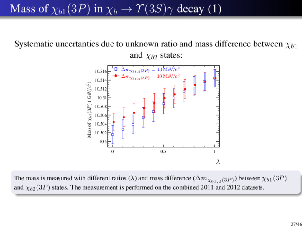
27. Mass of χb1 (3P) in χb → Υ(3S)γ decay (1) Systematic uncertanties due to unknown ratio and mass difference between χb1 and χb2 states: 0 0.5 1 10.5 10.502 10.504 10.506 10.508 10.51 10.512 10.514 10.516 Mass of χb1(3P) ( GeV/c2) λ ∆mχb1,2(3P ) = 13 MeV/c2 ∆mχb1,2(3P ) = 10 MeV/c2 The mass is measured with different ratios (λ) and mass difference (∆mχb1,2(3P )) between χb1(3P) and χb2(3P) states. The measurement is performed on the combined 2011 and 2012 datasets. 27/46
28. Mass of χb1 (3P) in χb → Υ(3S)γ decay (2) The measured mχb1(3P)=10,508 ± 2 (stat) ± 8 (syst) MeV/c2 is consistent with the mass measured in another study with converted photons — 10,510 ± 3.0 (stat)+4.4 −3.4 (syst) MeV/c2 (very preliminary results). ATLAS measured χb1 and χb2 mass barycenter for mχb2 − mχb1 = 12 MeV/c2 and λ = 0.5: mχb(3P) = 10,530 ± 5 (stat) ± 9 (syst) MeV/c2 D0: mχb(3P) = 10,551 ± 14 (stat) ± 17 (syst) MeV/c2 28/46
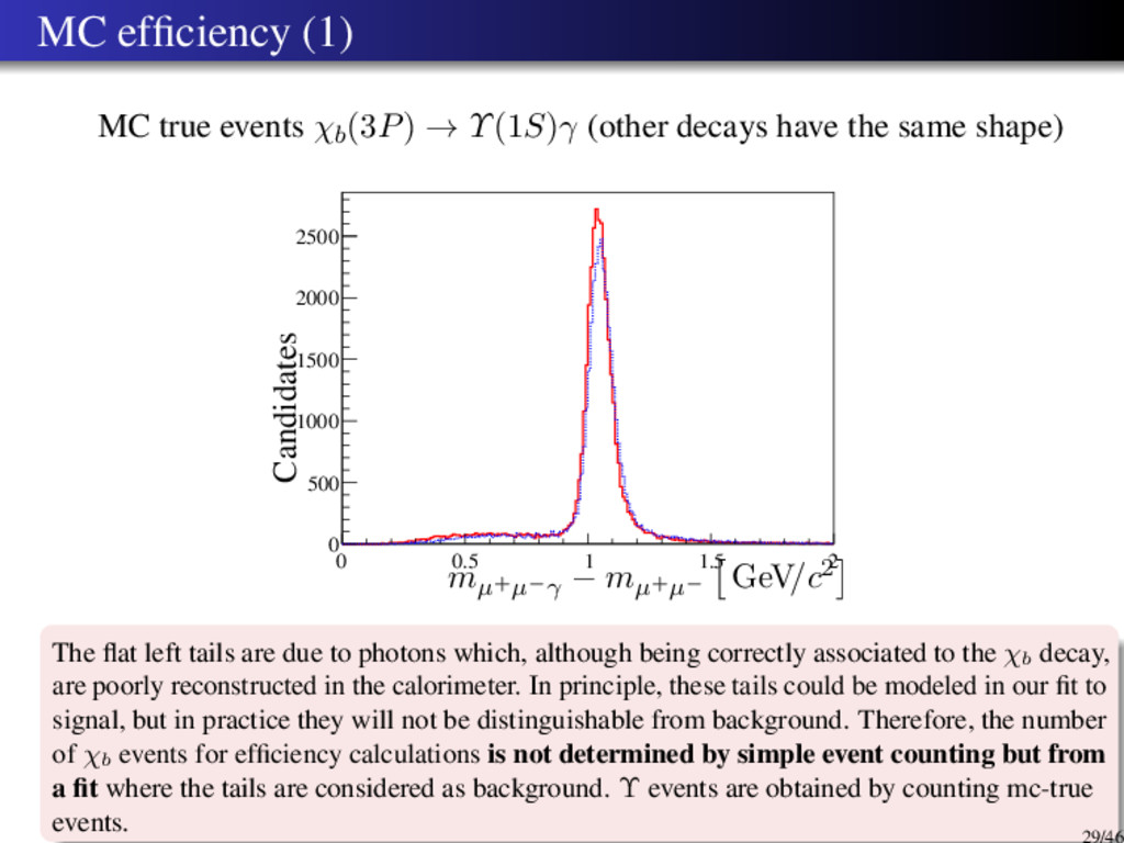
29. MC efficiency (1) MC true events χb(3P) → Υ(1S)γ (other decays have the same shape) 0 0.5 1 1.5 2 0 500 1000 1500 2000 2500 Candidates mµ+µ−γ − mµ+µ− GeV/c2 The flat left tails are due to photons which, although being correctly associated to the χb decay, are poorly reconstructed in the calorimeter. In principle, these tails could be modeled in our fit to signal, but in practice they will not be distinguishable from background. Therefore, the number of χb events for efficiency calculations is not determined by simple event counting but from a fit where the tails are considered as background. Υ events are obtained by counting mc-true events. 29/46
30. Monte-Carlo photon reconstruction (2) Example of fits: 9.8 9.9 10 10.1 0 1000 2000 3000 4000 5000 6000 -4 -2 0 2 4 χb1(1P) → Υ(1S)γ 6 < pΥ (1S) T < 40 GeV/c mµ+µ−γ − mµ+µ− + mPDG Υ(1S) GeV/c2 Candidates/(10 MeV/c2) 10 10.2 10.4 10.6 0 500 1000 1500 2000 2500 -4 -2 0 2 4 χb1(2P) → Υ(1S)γ 6 < pΥ (1S) T < 40 GeV/c mµ+µ−γ − mµ+µ− + mPDG Υ(1S) GeV/c2 Candidates/(10 MeV/c2) 10.2 10.4 10.6 10.8 0 200 400 600 800 1000 1200 1400 -4 -2 0 2 4 χb1(3P) → Υ(1S)γ 6 < pΥ (1S) T < 40 GeV/c mµ+µ−γ − mµ+µ− + mPDG Υ(1S) GeV/c2 Candidates/(10 MeV/c2) 10.2 10.25 10.3 0 10 20 30 40 50 -4 -2 0 2 4 χb1(2P) → Υ(2S)γ 18 < pΥ (2S) T < 40 GeV/c mµ+µ−γ − mµ+µ− + mPDG Υ(2S) GeV/c2 Candidates/(10 MeV/c2) 10.4 10.5 10.6 0 20 40 60 80 100 120 -4 -2 0 2 4 χb1(3P) → Υ(2S)γ 18 < pΥ (2S) T < 40 GeV/c mµ+µ−γ − mµ+µ− + mPDG Υ(2S) GeV/c2 Candidates/(10 MeV/c2) 10.45 10.5 10.55 10.6 10.65 0 10 20 30 40 50 60 70 80 -4 -2 0 2 4 χb1(3P) → Υ(3S)γ 27 < pΥ (3S) T < 40 GeV/c mµ+µ−γ − mµ+µ− + mPDG Υ(3S) GeV/c2 Candidates/(10 MeV/c2) 30/46
31. Data — Monte Carlo comparison A comparison of the distribution of the relevant observables used in this analysis was performed on real and simulated data, in order to assess the reliability of Monte Carlo in computing efficiencies 0 0.2 0.4 0.6 0.8 1 0 0.01 0.02 0.03 0.04 0.05 0.06 0 0.2 0.4 0.6 0.8 1 0 0.01 0.02 0.03 0.04 0.05 0.06 0 0.2 0.4 0.6 0.8 1 -0.02 0 0.02 0.04 0.06 0.08 0.1 0 2 4 0 0.01 0.02 0.03 0.04 0.05 0.06 0.07 0.08 0 2 4 0 0.02 0.04 0.06 0.08 0 2 4 -0.02 0 0.02 0.04 0.06 0.08 0.1 0.12 0.14 0 10 20 30 0 0.01 0.02 0.03 0.04 0.05 0.06 0.07 0.08 0 10 20 30 0 0.02 0.04 0.06 0.08 0.1 0 10 20 30 -0.02 0 0.02 0.04 0.06 0.08 0.1 0.12 0.14 0.16 15 20 25 30 35 0 0.01 0.02 0.03 0.04 0.05 0.06 15 20 25 30 35 0 0.02 0.04 0.06 0.08 0.1 15 20 25 30 35 0 0.05 0.1 0.15 0.2 γ confidence level γ confidence level γ confidence level χ2 of decay tree fitter χ2 of decay tree fitter χ2 of decay tree fitter pT [χb(1P)] GeV/c2 pT [χb(2P)] GeV/c2 pT [χb(3P)] GeV/c2 pT [Υ(1S)] GeV/c2 pT [Υ(1S)] GeV/c2 pT [Υ(1S)] GeV/c2 Arbitrary units Arbitrary units Arbitrary units Arbitrary units Arbitrary units Arbitrary units Arbitrary units Arbitrary units Arbitrary units Arbitrary units Arbitrary units Arbitrary units χb(1P) χb(2P) χb(3P) χb(1P) χb(2P) χb(3P) χb(1P) χb(2P) χb(3P) χb(1P) χb(2P) χb(3P) The agreement is generally very good. 31/46
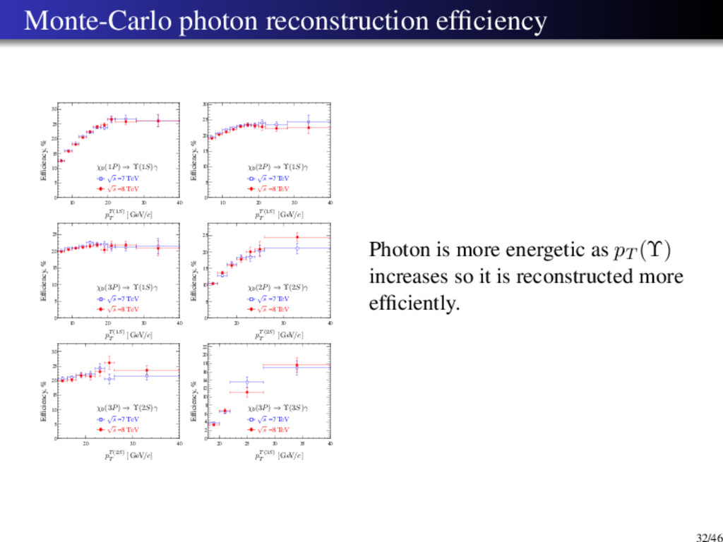
32. Monte-Carlo photon reconstruction efficiency 20 30 40 0 5 10 15 20 25 30 Efficiency, % pΥ(2S) T [ GeV/c] χb(3P) → Υ(2S)γ √ s =7 TeV √ s =8 TeV 20 25 30 35 40 0 2 4 6 8 10 12 14 16 18 20 22 Efficiency, % pΥ(3S) T [ GeV/c] χb(3P) → Υ(3S)γ √ s =7 TeV √ s =8 TeV 10 20 30 40 0 5 10 15 20 25 Efficiency, % pΥ(1S) T [ GeV/c] χb(3P) → Υ(1S)γ √ s =7 TeV √ s =8 TeV 20 30 40 0 5 10 15 20 25 Efficiency, % pΥ(2S) T [ GeV/c] χb(2P) → Υ(2S)γ √ s =7 TeV √ s =8 TeV 10 20 30 40 0 5 10 15 20 25 30 Efficiency, % pΥ(1S) T [ GeV/c] χb(1P) → Υ(1S)γ √ s =7 TeV √ s =8 TeV 10 20 30 40 0 5 10 15 20 25 30 Efficiency, % pΥ(1S) T [ GeV/c] χb(2P) → Υ(1S)γ √ s =7 TeV √ s =8 TeV Photon is more energetic as pT (Υ) increases so it is reconstructed more efficiently. 32/46
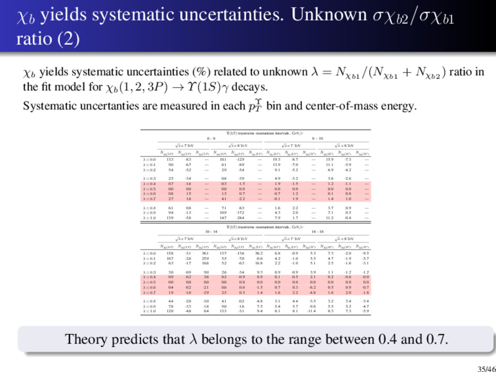
33. Systematic uncertainties Since this analysis measures the fraction of Υ(nS) particles originating from χb decays, most systematic uncertainties cancel in the ratio and only residual effects need to be taken into account. Systematic uncertainties on the event yields are mostly due to the fit model of Υ and χb invariant masses, while the ones on the efficiency are due to the photon reconstruction and the unknown initial polarization of χb and Υ particles. 33/46
34. χb yields systematic uncertainties. Unknown σχb2 /σχb1 ratio (1) The σ(χb2)/σ(χb1) ratio prediction: CDF LHCb Χb scaled Χb Χc CMS preliminary 5 10 15 20 25 30 0.0 0.5 1.0 1.5 2.0 2.5 3.0 pT , GeV σ(χ2)/σ(χ1) Transverse momentum distributions of the dσ [χ2 ] /dσ[χ1 ] ratio. Solid and dashed lines stand for charmonium and bottomonium mesons. The dot-dashed line corresponds to the rescaled bottomonium ratio: σb2 /σb1 (Mχc /Mχb pT ). The experimental results for charmonium from LHCb are shown with dots, CDF — with rectangles, and CMS — with triangles. 34/46
35. χb yields systematic uncertainties. Unknown σχb2 /σχb1 ratio (2) χb yields systematic uncertainties (%) related to unknown λ = Nχb1 /(Nχb1 + Nχb2 ) ratio in the fit model for χb (1, 2, 3P) → Υ(1S)γ decays. Systematic uncertanties are measured in each pΥ T bin and center-of-mass energy. Υ(1S) transverse momentum intervals, GeV/c 6 – 8 8 – 10 √ s = 7 TeV √ s = 8 TeV √ s = 7 TeV √ s = 8 TeV Nχb(1P) Nχb(2P) Nχb(3P) Nχb(1P) Nχb(2P) Nχb(3P) Nχb(1P) Nχb(2P) Nχb(3P) Nχb(1P) Nχb(2P) Nχb(3P) λ = 0.0 13.3 -8.3 — 10.1 -12.9 — 19.3 -8.7 — 15.9 -7.3 — λ = 0.1 9.0 -6.7 — 6.1 -8.9 — 13.9 -7.0 — 11.1 -5.9 — λ = 0.2 5.4 -5.2 — 2.9 -5.4 — 9.1 -5.2 — 6.9 -4.2 — λ = 0.3 2.5 -3.4 — 0.8 -3.9 — 4.9 -3.2 — 3.6 -2.6 — λ = 0.4 0.7 -1.6 — -0.3 -1.5 — 1.9 -1.5 — 1.2 -1.1 — λ = 0.5 0.0 0.0 — 0.0 0.0 — 0.0 0.0 — 0.0 0.0 — λ = 0.6 0.8 1.5 — 1.3 0.7 — -0.7 1.2 — 0.1 0.8 — λ = 0.7 2.7 1.6 — 4.1 -2.2 — -0.1 1.9 — 1.4 1.0 — λ = 0.8 6.1 0.8 — 7.1 -8.3 — 1.6 2.2 — 3.7 0.9 — λ = 0.9 9.4 -1.3 — 10.9 -17.2 — 4.3 2.0 — 7.1 0.5 — λ = 1.0 13.9 -5.8 — 14.7 -24.4 — 7.9 1.7 — 11.2 -0.4 — Υ(1S) transverse momentum intervals, GeV/c 10 – 14 14 – 18 √ s = 7 TeV √ s = 8 TeV √ s = 7 TeV √ s = 8 TeV Nχb(1P) Nχb(2P) Nχb(3P) Nχb(1P) Nχb(2P) Nχb(3P) Nχb(1P) Nχb(2P) Nχb(3P) Nχb(1P) Nχb(2P) Nχb(3P) λ = 0.0 15.8 -3.1 36.1 13.7 -13.6 36.2 6.8 -0.9 5.3 7.3 -2.0 -9.5 λ = 0.1 10.7 -2.6 25.9 5.5 -7.0 -0.6 4.2 -1.0 5.5 4.7 -1.9 -5.7 λ = 0.2 6.3 -1.7 16.6 5.2 -6.3 16.8 2.2 -1.0 5.1 2.5 -1.6 -3.1 λ = 0.3 3.0 -0.9 9.0 2.6 -3.4 9.3 0.9 -0.9 3.9 1.1 -1.2 -1.2 λ = 0.4 0.9 -0.2 3.6 0.2 -0.9 0.9 0.1 -0.5 2.1 0.2 -0.6 -0.0 λ = 0.5 0.0 0.0 0.0 0.0 0.0 0.0 0.0 0.0 0.0 0.0 0.0 0.0 λ = 0.6 0.4 -0.2 -2.1 0.6 0.6 -1.5 0.7 0.3 -6.2 0.5 0.9 -0.7 λ = 0.7 1.9 -1.0 -2.9 2.5 0.3 1.4 1.6 2.2 -4.8 1.6 2.0 -1.8 λ = 0.8 4.4 -2.0 -3.0 4.1 -0.2 -4.8 3.1 4.4 -3.5 3.2 3.4 -3.4 λ = 0.9 7.8 -3.3 -1.8 9.0 -1.6 7.5 5.4 5.7 -9.6 5.5 5.2 -4.7 λ = 1.0 12.0 -4.8 0.4 13.3 -3.1 9.4 8.1 8.1 -11.4 8.3 7.3 -5.9 Theory predicts that λ belongs to the range between 0.4 and 0.7. 35/46
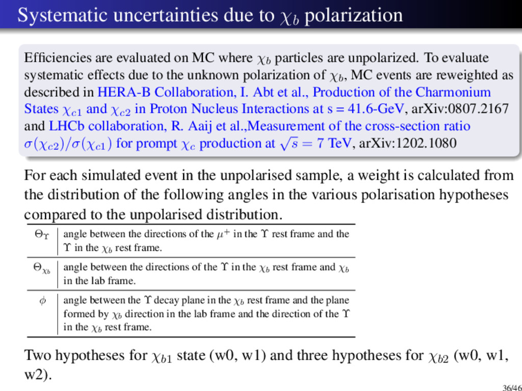
36. Systematic uncertainties due to χb polarization Efficiencies are evaluated on MC where χb particles are unpolarized. To evaluate systematic effects due to the unknown polarization of χb, MC events are reweighted as described in HERA-B Collaboration, I. Abt et al., Production of the Charmonium States χc1 and χc2 in Proton Nucleus Interactions at s = 41.6-GeV, arXiv:0807.2167 and LHCb collaboration, R. Aaij et al.,Measurement of the cross-section ratio σ(χc2 )/σ(χc1 ) for prompt χc production at √ s = 7 TeV, arXiv:1202.1080 For each simulated event in the unpolarised sample, a weight is calculated from the distribution of the following angles in the various polarisation hypotheses compared to the unpolarised distribution. ΘΥ angle between the directions of the µ+ in the Υ rest frame and the Υ in the χb rest frame. Θχb angle between the directions of the Υ in the χb rest frame and χb in the lab frame. φ angle between the Υ decay plane in the χb rest frame and the plane formed by χb direction in the lab frame and the direction of the Υ in the χb rest frame. Two hypotheses for χb1 state (w0, w1) and three hypotheses for χb2 (w0, w1, w2). 36/46
37. Systematic uncertainties due to χb polarization The ratio of efficiency for unpolarized χb to efficiency for polarized χb. 10 20 30 40 0.99 0.995 1 1.005 1.01 1.015 1.02 1.025 1.03 1.035 10 20 30 40 0.985 0.99 0.995 1 1.005 1.01 pΥ(1S) T [ GeV/c] pΥ(1S) T [ GeV/c] pΥ(1S) T [ GeV/c] pΥ(1S) T [ GeV/c] εmχb1 /εunpol εmχb1 /εunpol χb1 (1P) → Υ(1S)γ |mχb1 | = 0 χb1 (1P) → Υ(1S)γ |mχb1 | = 1 The difference between ratio and 1 is considered as systematic uncertainty. 37/46
38. Summary of systematic uncertainties Υ fraction uncertainties common to all χb decays (%) Υ fit model ±0.7 γ reconstruction ±3 Summary of Υ fraction systematic uncertainties (%) (maximum deviations that were found in pΥ T bins): χb fit model χb polarization χb(1P) → Υ(1S)γ +4.3 −5.8 +5.1 −4.0 χb(2P) → Υ(1S)γ +4.8 −6.2 +5.8 −6.8 χb(3P) → Υ(1S)γ +19.6 −16.6 +6.9 −6.7 χb(2P) → Υ(2S)γ +2.3 −7.0 +8.7 −7.8 χb(3P) → Υ(2S)γ +19.7 −19.9 +4.5 −4.2 χb(3P) → Υ(3S)γ +20.9 −27.6 +6.4 −7.5 38/46
39. Υ fractions in χb → Υγ decays 10 20 30 40 0 5 10 15 20 25 30 35 40 45 50 Υ(1S) fraction, % pΥ(1S) T [ GeV/c] χb(1P) → Υ(1S)γ √ s =7 TeV √ s =8 TeV 10 20 30 40 0 5 10 15 20 25 30 35 40 45 50 Υ(1S) fraction, % pΥ(1S) T [ GeV/c] χb(2P) → Υ(1S)γ √ s =7 TeV √ s =8 TeV 10 20 30 40 0 5 10 15 20 25 30 35 40 45 50 Υ(1S) fraction, % pΥ(1S) T [ GeV/c] χb(3P) → Υ(1S)γ √ s =7 TeV √ s =8 TeV 10 20 30 40 0 5 10 15 20 25 30 35 40 45 50 Υ(2S) fraction, % pΥ(2S) T [ GeV/c] χb(2P) → Υ(2S)γ √ s =7 TeV √ s =8 TeV 10 20 30 40 0 5 10 15 20 25 30 35 40 45 50 Υ(2S) fraction, % pΥ(2S) T [ GeV/c] χb(3P) → Υ(2S)γ √ s =7 TeV √ s =8 TeV 10 20 30 40 0 10 20 30 40 50 60 70 80 90 100 Υ(3S) fraction, % pΥ(3S) T [ GeV/c] χb(3P) → Υ(3S)γ √ s =7 TeV √ s =8 TeV 10 20 30 40 0 5 10 15 20 25 30 35 40 45 50 Υ(1S) fraction, % pΥ(1S) T [ GeV/c] χb(1P) → Υ(1S)γ √ s =7 TeV √ s =8 TeV √ s =7 TeV (2010) Outer error bars show statistical and systematics errors, inner error bars — only statistical errors. 39/46
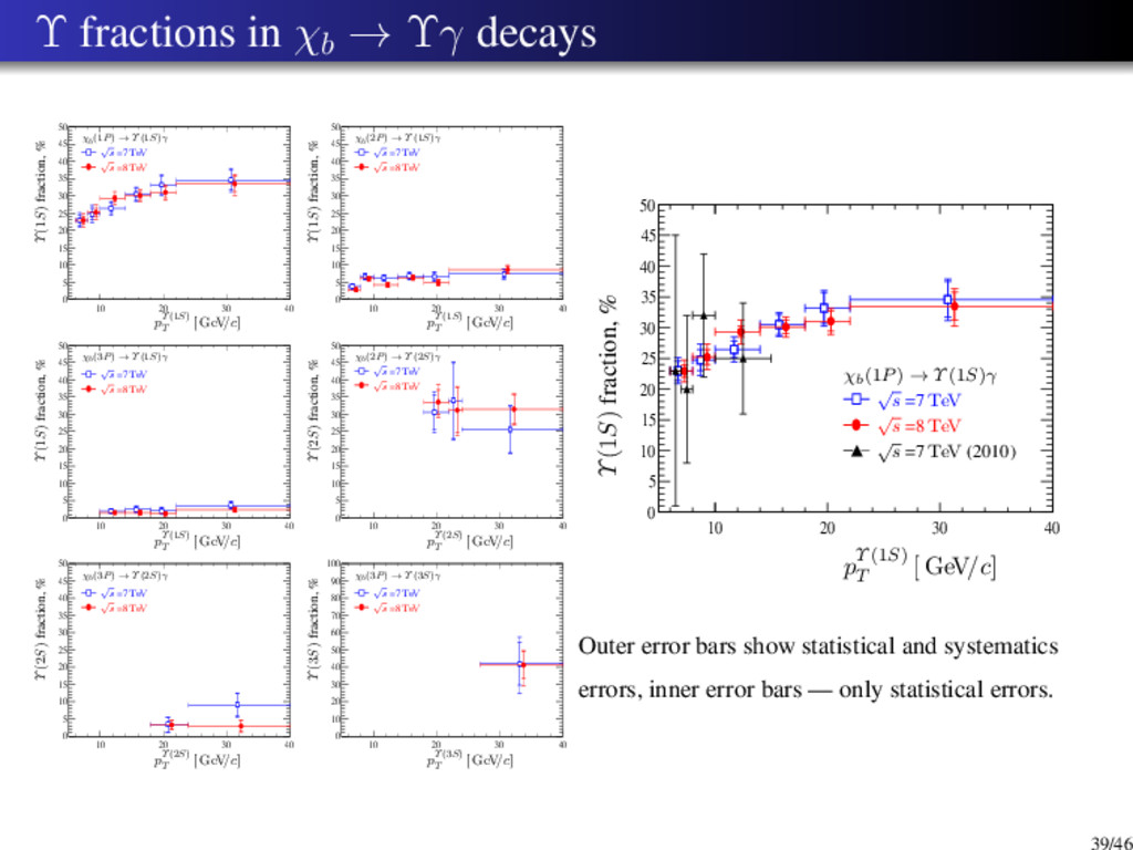
40. Summary Measured fractions of Υ(1, 2, 3S) originated from χb decays. About 40% of Υ come from χb, with mild dependence on Υ transverse momentum. This analysis improves significantly the statistical precision of the previous work and adds more decays and transverse momentum regions. The LHCb detector design allows to perform measurements in Υ rapidity and transverse momentum regions, which are complementary to the ones exploited by ATLAS and CMS. Measured mass of χb(3P) is 10, 508 ± 2 (stat) ± 8 (stat) MeV/c2, consistent with another determination which uses converted photons. A software profiling tool was developed. The results on χb production were regularly presented at the LHCb bottomonium working group, an internal document was prepared by the author, is currently under review and will form the basis of a future LHCb publication. 40/46
41. High Level Trigger software performance profiling 41/46
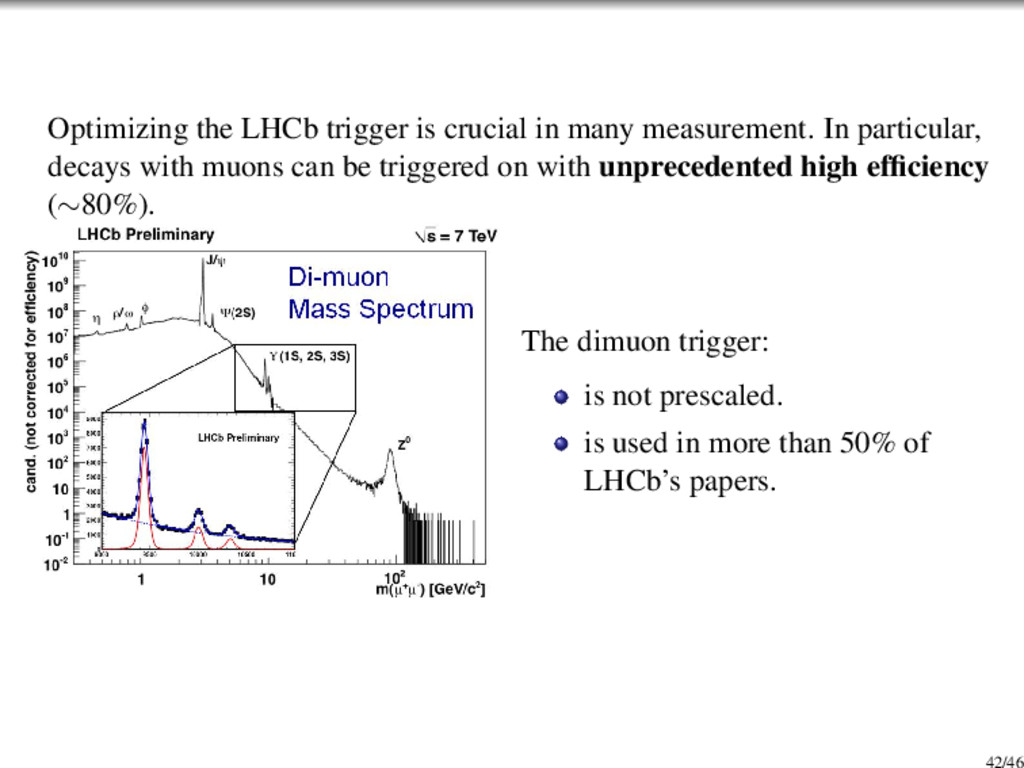
42. Optimizing the LHCb trigger is crucial in many measurement. In particular, decays with muons can be triggered on with unprecedented high efficiency (∼80%). The dimuon trigger: is not prescaled. is used in more than 50% of LHCb’s papers. 42/46
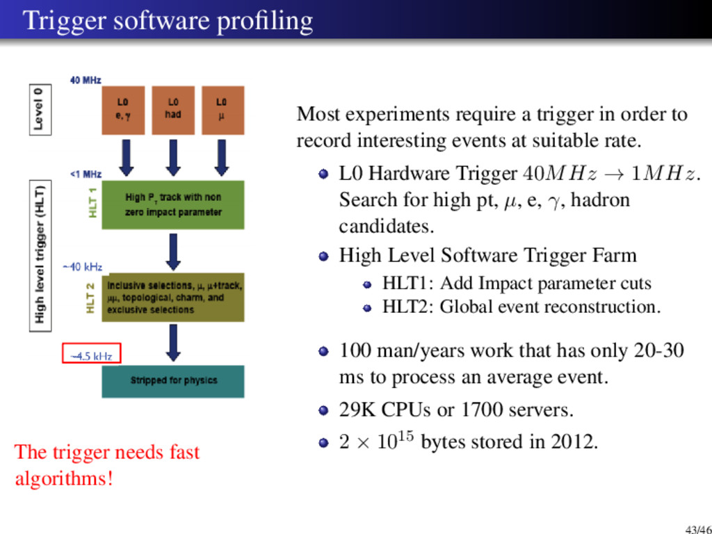
43. Trigger software profiling The trigger needs fast algorithms! Most experiments require a trigger in order to record interesting events at suitable rate. L0 Hardware Trigger 40MHz → 1MHz. Search for high pt, µ, e, γ, hadron candidates. High Level Software Trigger Farm HLT1: Add Impact parameter cuts HLT2: Global event reconstruction. 100 man/years work that has only 20-30 ms to process an average event. 29K CPUs or 1700 servers. 2 × 1015 bytes stored in 2012. 43/46
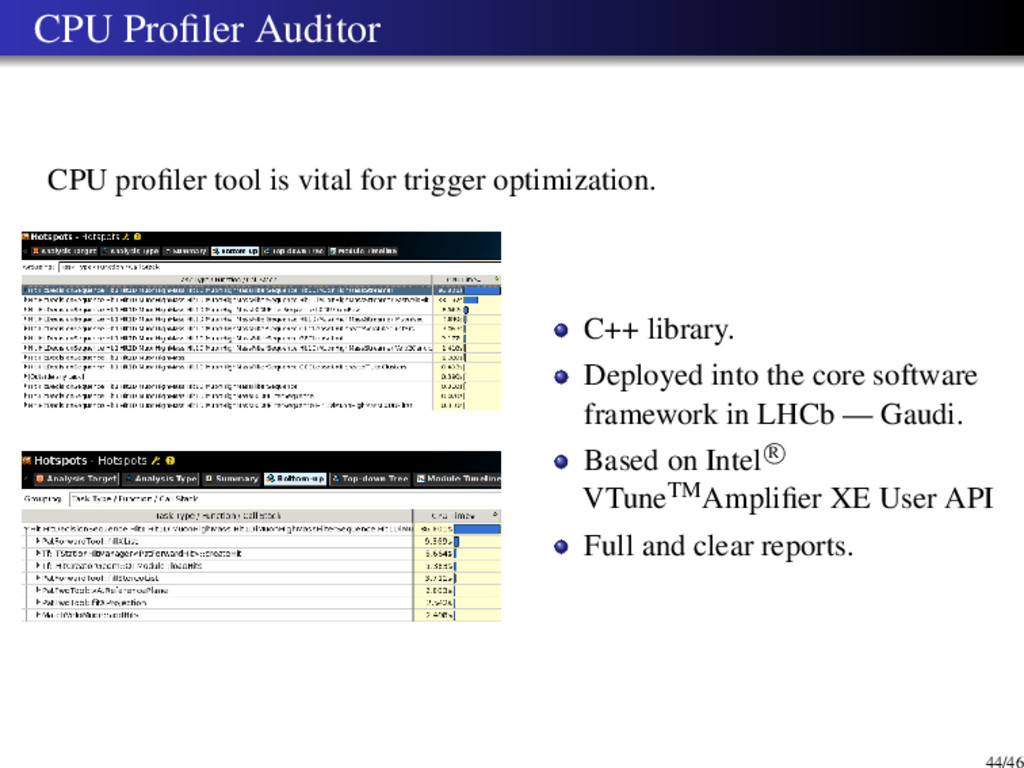
44. CPU Profiler Auditor CPU profiler tool is vital for trigger optimization. C++ library. Deployed into the core software framework in LHCb — Gaudi. Based on Intel R VTuneTMAmplifier XE User API Full and clear reports. 44/46
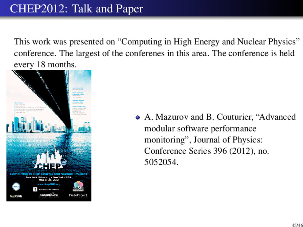
45. CHEP2012: Talk and Paper This work was presented on “Computing in High Energy and Nuclear Physics” conference. The largest of the conferenes in this area. The conference is held every 18 months. A. Mazurov and B. Couturier, “Advanced modular software performance monitoring”, Journal of Physics: Conference Series 396 (2012), no. 5052054. 45/46
46. Thank you! 46/46