Ferrara 2013

Talk at Ferrara on 16 Dec 2013 (unofficial results)

Transcript

1. Study of χb production at √ s =7 and 8 TeV LHCb (CERN) Sasha Mazurov University of Ferrara (Italy) & CERN 16 December 2013 1/34
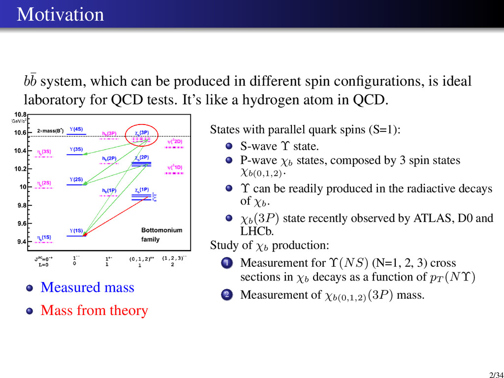
2. Motivation b¯ b system, which can be produced in different spin configurations, is ideal laboratory for QCD tests. It’s like a hydrogen atom in QCD. Measured mass Mass from theory States with parallel quark spins (S=1): S-wave Υ state. P-wave χb states, composed by 3 spin states χb(0,1,2) . Υ can be readily produced in the radiactive decays of χb. χb (3P) state recently observed by ATLAS, D0 and LHCb. Study of χb production: 1 Measurement for Υ(NS) (N=1, 2, 3) cross sections in χb decays as a function of pT (NΥ) 2 Measurement of χb(0,1,2) (3P) mass. 2/34
3. Previous analysis at LHCb ”Measurement of the fraction of Υ(1S) originating from χb(1P) in pp collisions at √ s =7 TeV ”, arXiv:1209.0282, L = 32 pb−1 ”Observation of the χb(3P) state at LHCb in pp collisions at √ s =7 TeV ”, LHCb-CONF-2012-020, L = 0.9 fb−1. 3/34
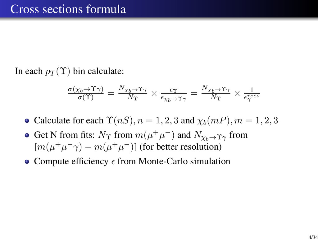
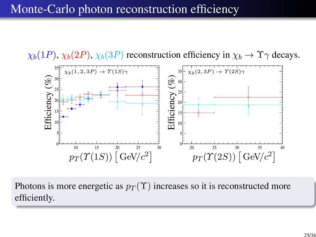
4. Cross sections formula In each pT (Υ) bin calculate: σ(χb→Υγ) σ(Υ) = Nχb→Υγ NΥ × Υ χb→Υγ = Nχb→Υγ NΥ × 1 reco γ Calculate for each Υ(nS), n = 1, 2, 3 and χb(mP), m = 1, 2, 3 Get N from fits: NΥ from m(µ+µ−) and Nχb→Υγ from [m(µ+µ−γ) − m(µ+µ−)] (for better resolution) Compute efficiency from Monte-Carlo simulation 4/34
5. Plan 1 Datasets 2 Determination of Υ yields 3 Determination of χb yields in the following decays χb (1, 2, 3P) → Υ(1S)γ χb (2, 3P) → Υ(2S)γ χb (3P) → Υ(3S)γ 4 Monte-Carlo efficiencies 5 The fraction of Υ originating from χb decays. 6 Systematic uncertainties 5/34
6. Datasets Full 2011 dataset at √ s =7 TeV. L = 1 fb−1 Full 2012 dataset at √ s =8 TeV. L = 2 fb−1 Monte-Carlo simulation of χb inclusive decays, generated 62 × 106 events. 6/34
7. The Υ selection Description Requirement Track fit quality χ2/ndf < 4 Track pT > 1 GeV/c Primary vertex probability > 0.5% Luminous region |zPV | < 0.5m and x2 PV + y2 PV < 100mm2 Kullback-Leibler distance > 5000 Muon and hadron hypotheses ∆ log Lµ−h > 0 Muon probability ProbNN > 0.5 Trigger lines: L0 DiMuon.*Decision HLT1 Hlt1DiMuonHighMass.*Decision HLT2 HLT2DiMuonB.*Decision 7/34
8. The Υ fit model 9 10 11 0 20 40 60 80 100 120 3 10 × -20 -10 0 10 20 Candidates/(40 MeV/c2) mµ+µ− GeV/c2 √ s = 7 TeV 6 < pµ+µ− T < 40 GeV/c 3 Crystal Ball functions for signal yields (α = 2, n = 5). Exponential function for combinatorial background. µ+µ− transverse momentum intervals ( GeV/c) 6 — 40 √ s = 7 TeV √ s = 8 TeV NΥ(1S) 284,300 ± 600 661,800 ± 900 NΥ(2S) 88,100 ± 400 204,800 ± 500 NΥ(3S) 50,850 ± 290 116,700 ± 400 B 294,300 ± 700 716,100 ± 1100 µΥ(1S) , MeV/c2 9456.64 ± 0.09 9455.24 ± 0.06 σΥ(1S) , MeV/c2 45.23 ± 0.08 45.38 ± 0.06 Υ(1S) mass is about 5 MeV/c2 lower than PDG value 9460.30 ± 0.26 MeV/c2 In this study Υ(1S) mass was fixed to 9.456 GeV/c2 8/34
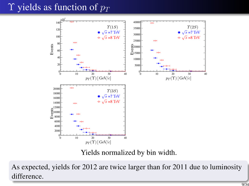
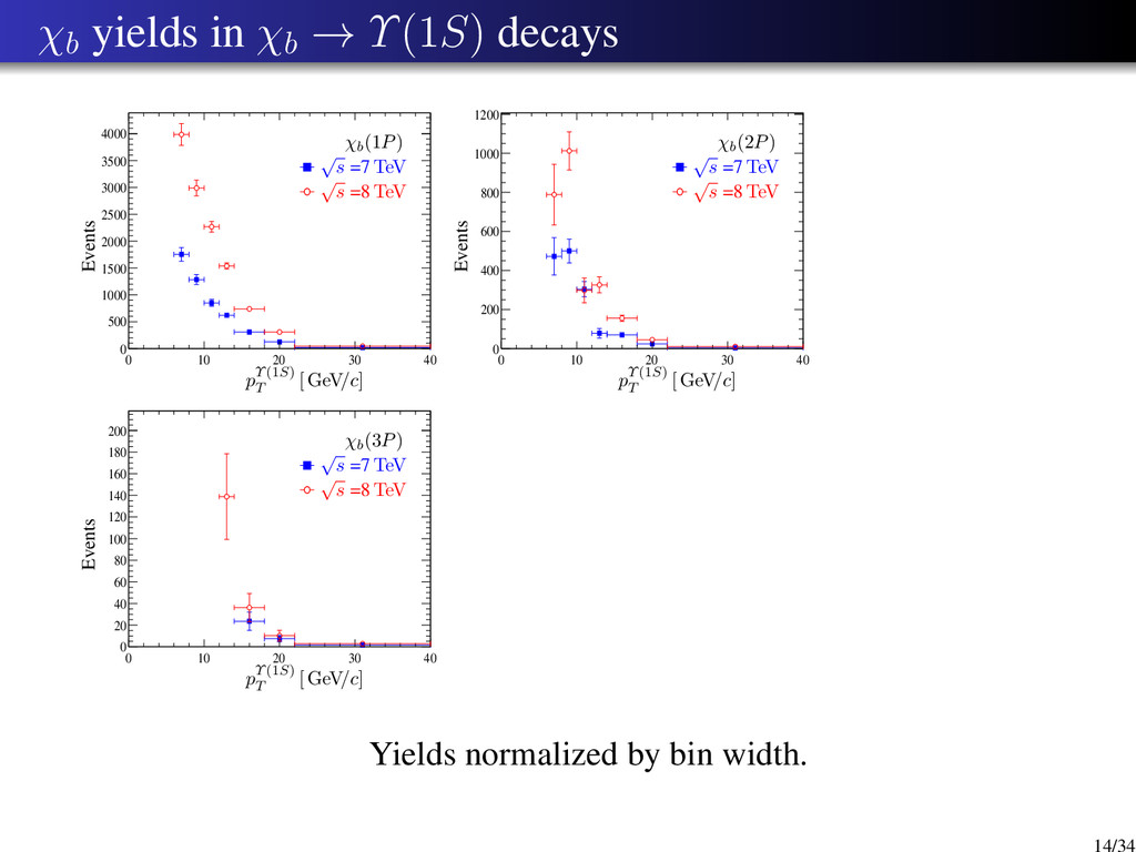
9. Υ yields as function of pT 0 10 20 30 40 0 2000 4000 6000 8000 10000 12000 14000 16000 18000 20000 0 10 20 30 40 0 20 40 60 80 100 120 140 3 10 × 0 10 20 30 40 0 5000 10000 15000 20000 25000 30000 35000 40000 Events pT (Υ) [ GeV/c] Υ(3S) Events pT (Υ) [ GeV/c] Υ(1S) Events pT (Υ) [ GeV/c] Υ(2S) √ s =7 TeV √ s =8 TeV √ s =7 TeV √ s =8 TeV √ s =7 TeV √ s =8 TeV Yields normalized by bin width. As expected, yields for 2012 are twice larger than for 2011 due to luminosity difference. 9/34
10. χb selection In this study photons reconstructed using the calorimeter information. Another approach is to track e+e− (converted photons) — this method has better invariant mass resolution, but requires more statistics. Cuts on γ: Transverse momentum of γ pT (γ) > 600 MeV/c Polar angle of γ in the µ+µ−γ rest frame cos θγ > 0 Confidence level of γ cl(γ) > 0.01 Dimuon mass windows: Decay Cut Description χb(1, 2, 3P) → Υ(1S) 9310 < µ+µ− < 9600 MeV/c 3σΥ(1S) < µ+µ− < 2.5σΥ(1S) MeV/c χb(2, 3P) → Υ(2S) 9870 < µ+µ− < 10090 MeV/c 3σΥ(2S) < µ+µ− < σΥ(2S) MeV/c χb(3P) → Υ(3S) 10300 < µ+µ− < 10526 MeV/c σΥ(3S) < µ+µ− < 3σΥ(3S) MeV/c 10/34
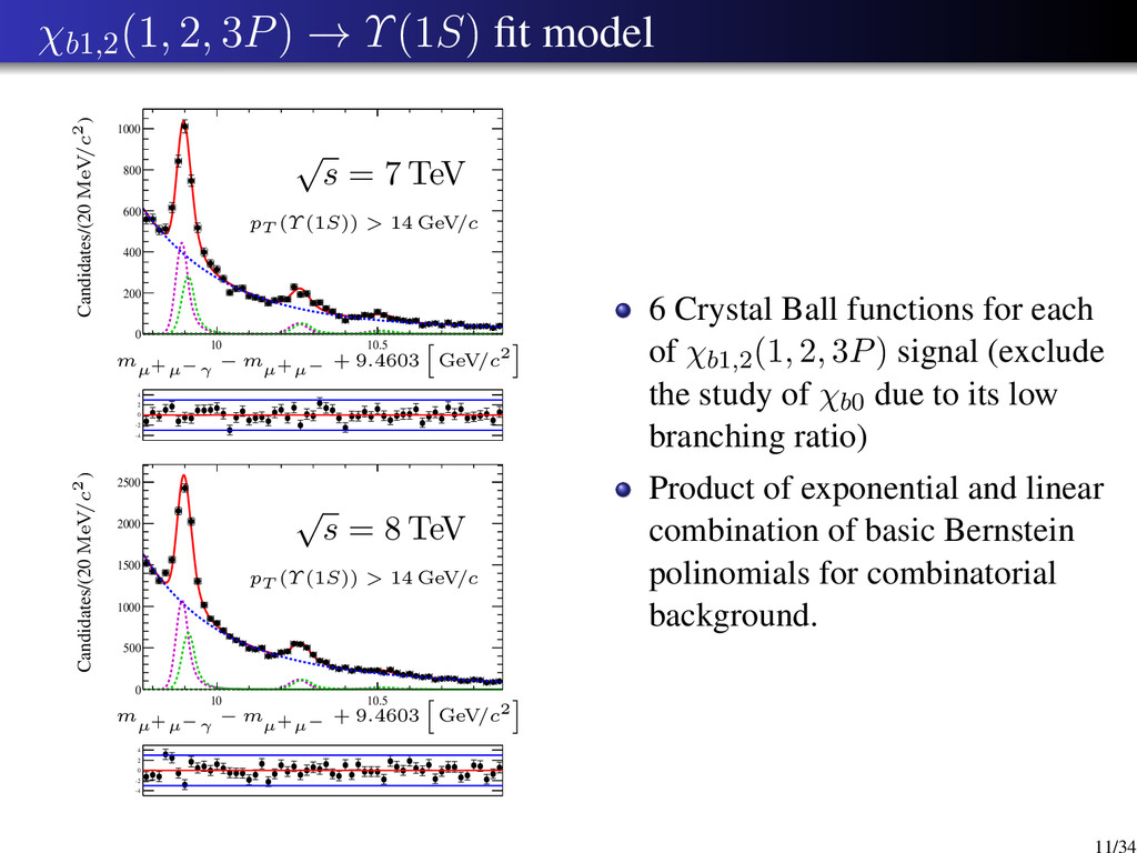
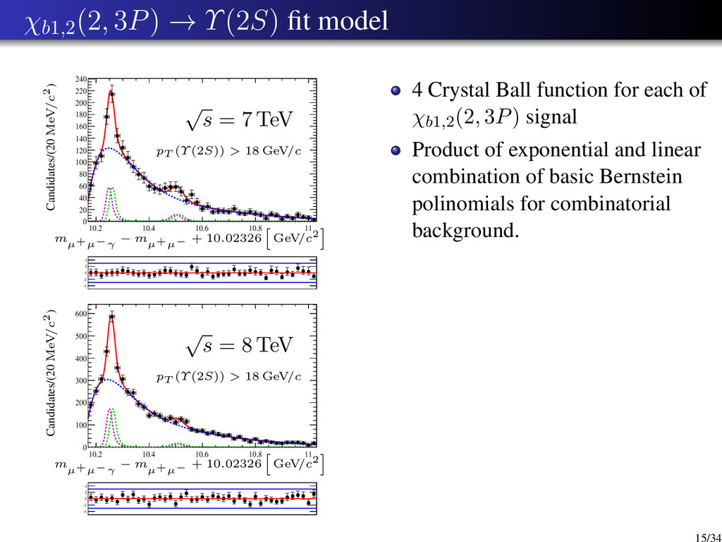
11. χb1,2 (1, 2, 3P) → Υ(1S) fit model 10 10.5 0 500 1000 1500 2000 2500 -4 -2 0 2 4 10 10.5 0 200 400 600 800 1000 -4 -2 0 2 4 Candidates/(20 MeV/c2) m µ+µ−γ − m µ+µ− + 9.4603 GeV/c2 √ s = 8 TeV pT (Υ (1S)) > 14 GeV/c Candidates/(20 MeV/c2) m µ+µ−γ − m µ+µ− + 9.4603 GeV/c2 √ s = 7 TeV pT (Υ (1S)) > 14 GeV/c 6 Crystal Ball functions for each of χb1,2(1, 2, 3P) signal (exclude the study of χb0 due to its low branching ratio) Product of exponential and linear combination of basic Bernstein polinomials for combinatorial background. 11/34
12. χb1,2 (1, 2, 3P) → Υ(1S) fit model (2) Free parameters: µχb1(1P), yields and background parameters. Linked parameters for χb1 and χb2 signals: µχb2(jP ) = µχb1(jP ) + ∆mP DG χb2(jP ) , j=1,2 µχb2(3P ) = µχb1(3P ) + ∆mtheory χb2(3P ) Nχb = λNχb1 + (1 − λ)Nχb2 σχb2 = σχb1 Other linked parameters: µχb1(2P ) = µχb1(1P ) + ∆mP DG χb1(2P ) µχb1(3P ) = µχb1(1P ) + ∆mχb1(3P ) (∆mχb1(3P ) measured in this study) Fixed parameters from MC study: σχb1(1P ) scaled by 1.17, σχb1(2P ) σχb1(1P ) , σχb1(3P ) σχb1(1P ) α and n parameters of CB. Υ(1S) transverse momentum intervals pT (Υ) > 14 GeV/c √ s = 7 TeV √ s = 8 TeV Nχb(1P) 1960 ± 70 4730 ± 120 Nχb(2P) 410 ± 40 930 ± 70 Nχb(3P) 154 ± 34 220 ± 50 B 9230 ± 120 24,870 ± 200 µχb1(1P) , MeV/c2 9890.9 ± 1.0 9891.6 ± 0.7 ∆mχb1(2P) , MeV/c2 363 ∆mχb1(3P) , MeV/c2 614 ∆mPDG χb2,1(1P) , MeV/c2 19.43 ∆mPDG χb2,1(2P) , MeV/c2 13.19 ∆mtheory χb2,1(2P) , MeV/c2 13.00 σχb1(1P) , MeV/c2 19.02 σχb2(1P) /σχb1(1P) , MeV/c2 1.05 σχb1(2P) /σχb1(1P) , MeV/c2 1.50 σχb1(3P) /σχb1(1P) , MeV/c2 2.00 λχb(1P) 0.6 λχb(2P) 0.5 λχb(3P) 0.5 αχb(1P) -1.10 αχb(2P) -1.10 αχb(3P) -1.25 nχb(1P) 5.0 nχb(2P) 5.0 nχb(3P) 5.0 τ -2.5 ± 0.5 -3.02 ± 0.30 c0 -0.10 ± 0.11 0.02 ± 0.06 c1 1.36 ± 0.04 0.25 ± 0.04 χ2/n.d.f 1.2 1.5 Good agreement between µχb1(1P ) and value in PDG (9892 MeV/c2). 12/34
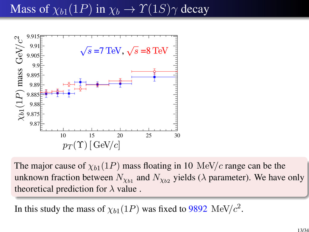
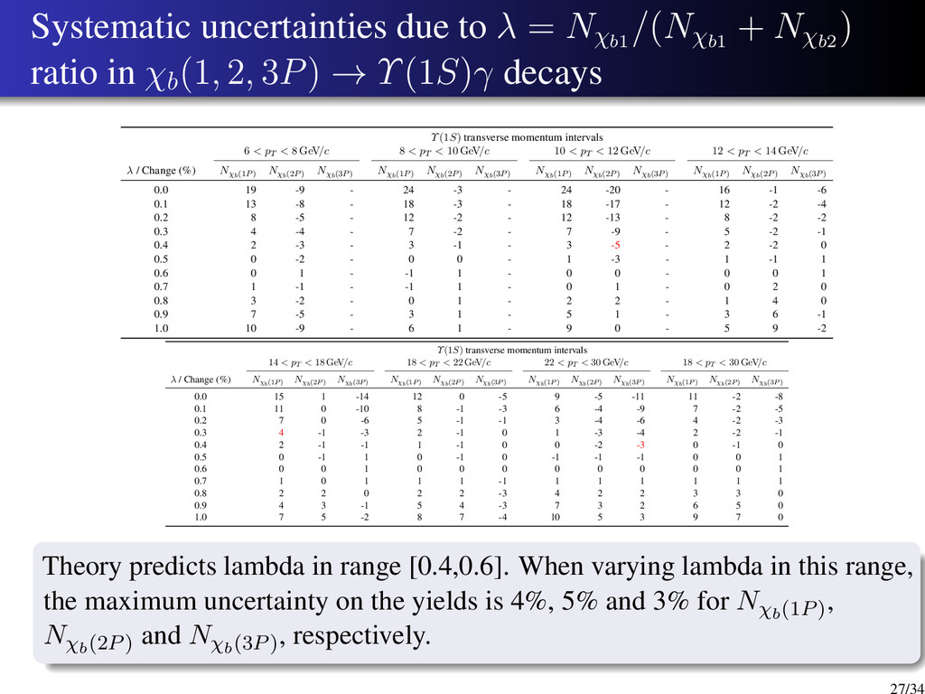
13. Mass of χb1 (1P) in χb → Υ(1S)γ decay 10 15 20 25 30 9.87 9.875 9.88 9.885 9.89 9.895 9.9 9.905 9.91 9.915 √ s =7 TeV, √ s =8 TeV √ s =7 TeV, √ s =8 TeV χb1(1P) mass GeV/c2 pT (Υ) [ GeV/c] The major cause of χb1(1P) mass floating in 10 MeV/c range can be the unknown fraction between Nχb1 and Nχb2 yields (λ parameter). We have only theoretical prediction for λ value . In this study the mass of χb1(1P) was fixed to 9892 MeV/c2. 13/34
14. χb yields in χb → Υ(1S) decays 0 10 20 30 40 0 20 40 60 80 100 120 140 160 180 200 0 10 20 30 40 0 500 1000 1500 2000 2500 3000 3500 4000 0 10 20 30 40 0 200 400 600 800 1000 1200 Events pΥ(1S) T [ GeV/c] χb(3P) Events pΥ(1S) T [ GeV/c] χb(1P) Events pΥ(1S) T [ GeV/c] χb(2P) √ s =7 TeV √ s =8 TeV √ s =7 TeV √ s =8 TeV √ s =7 TeV √ s =8 TeV Yields normalized by bin width. 14/34
15. χb1,2 (2, 3P) → Υ(2S) fit model 10.2 10.4 10.6 10.8 11 0 100 200 300 400 500 600 -4 -2 0 2 4 10.2 10.4 10.6 10.8 11 0 20 40 60 80 100 120 140 160 180 200 220 240 -4 -2 0 2 4 Candidates/(20 MeV/c2) m µ+µ−γ − m µ+µ− + 10.02326 GeV/c2 √ s = 8 TeV pT (Υ (2S)) > 18 GeV/c Candidates/(20 MeV/c2) m µ+µ−γ − m µ+µ− + 10.02326 GeV/c2 √ s = 7 TeV pT (Υ (2S)) > 18 GeV/c 4 Crystal Ball function for each of χb1,2(2, 3P) signal Product of exponential and linear combination of basic Bernstein polinomials for combinatorial background. 15/34
16. χb1,2 (2, 3P) → Υ(2S) fit model (2) Free parameters: µχb1(2P), yields and background parameters. Linked parameters for χb1 and χb2 signals: µχb2(2P ) = µχb1(2P ) + ∆mP DG χb2(2P ) µχb2(3P ) = µχb1(3P ) + ∆mtheory χb2(3P ) Nχb = λNχb1 + (1 − λ)Nχb2 σχb2 = σχb1 Other linked parameters: µχb1(3P ) = µχb1(1P ) + ∆mχb1(3P ) (∆mχb1(3P ) measured in this study) Fixed parameters from MC study: σχb1(2P ) , σχb1(3P ) σχb1(2P ) α and n parameters of CB. Υ(2S) transverse momentum intervals pT (Υ(2S)) > 18 GeV/c √ s = 7 TeV √ s = 8 TeV Nχb(2P) 185 ± 30 550 ± 50 Nχb(3P) 64 ± 19 93 ± 29 B 1800 ± 50 4590 ± 80 µχb1(2P) , MeV/c2 10,248.3 ± 2.3 10,250.4 ± 1.3 ∆mχb1(3P) , MeV/c2 252 ∆mPDG χb2,1(2P) , MeV/c2 13.19 ∆mχb2,1(3P) , MeV/c2 13.00 σχb1(2P) , MeV/c2 11.58 σχb1(3P) /σχb1(2P) , MeV/c2 1.84 λχb(2P) 0.5 λχb(3P) 0.5 αχb(2P) -1.10 αχb(3P) -1.25 nχb(2P) 5.0 nχb(3P) 5.0 τ -8.3 ± 2.9 -8.6 ± 1.2 c0 0.40 ± 0.06 0.392 ± 0.030 c1 -2.30 ± 0.30 -2.35 ± 0.10 c2 -2.6 ± 0.6 -2.67 ± 0.13 c3 0.3 ± 0.6 0.36 ± 0.24 c4 - - χ2/n.d.f 0.6 1.0 The mass of χb1(2P ) is about 5 MeV/c2 less than value in PDG (10.25546 MeV/c2). 16/34
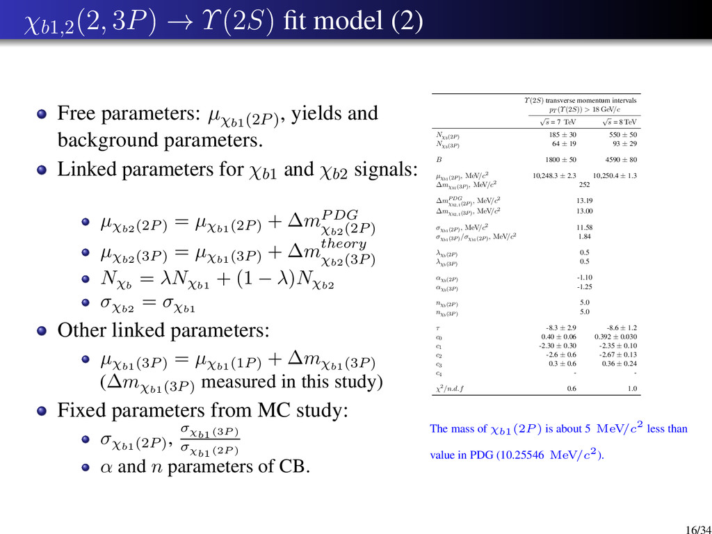
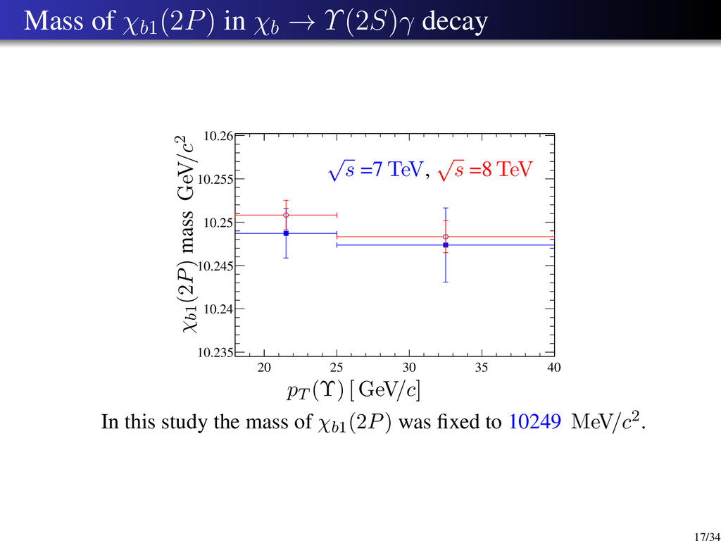
17. Mass of χb1 (2P) in χb → Υ(2S)γ decay 20 25 30 35 40 10.235 10.24 10.245 10.25 10.255 10.26 √ s =7 TeV, √ s =8 TeV χb1(2P) mass GeV/c2 pT (Υ) [ GeV/c] In this study the mass of χb1(2P) was fixed to 10249 MeV/c2. 17/34
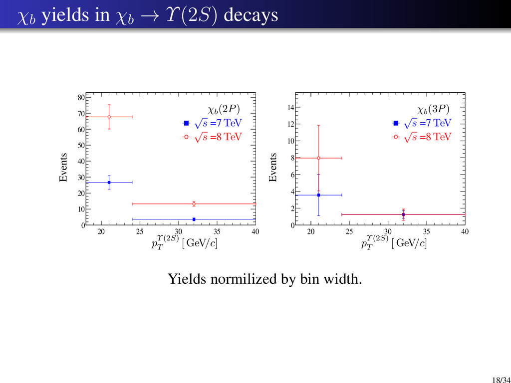
18. χb yields in χb → Υ(2S) decays 20 25 30 35 40 0 10 20 30 40 50 60 70 80 20 25 30 35 40 0 2 4 6 8 10 12 14 Events pΥ(2S) T [ GeV/c] χb(2P) Events pΥ(2S) T [ GeV/c] χb(3P) √ s =7 TeV √ s =8 TeV √ s =7 TeV √ s =8 TeV Yields normilized by bin width. 18/34
19. χb1,2 (3P) → Υ(3S) fit model 10.5 10.6 10.7 0 10 20 30 40 50 -4 -2 0 2 4 10.5 10.6 10.7 0 2 4 6 8 10 12 14 16 18 20 22 -4 -2 0 2 4 Candidates/(20 MeV/c2) m µ+µ−γ − m µ+µ− + 10.3552 GeV/c2 √ s = 8 GeV pT (Υ (3S)) > 27 GeV/c Candidates/(20 MeV/c2) m µ+µ−γ − m µ+µ− + 10.3552 GeV/c2 √ s = 7 GeV pT (Υ (3S)) > 27 GeV/c 2 Crystal Ball for each of χb1,2(3P) signal. Product of exponential and linear compination of basic Bernstein polinomials for combinatorial background. 19/34
20. χb1,2 (3P) → Υ(3S) fit model (2) Free parameters: µχb1(3P), yields and background parameters. Linked parameters for χb1 and χb2 signals: µχb2(3P ) = µχb1(3P ) + ∆mtheory χb2(3P ) Nχb = λNχb1 + (1 − λ)Nχb2 σχb2 = σχb1 Fixed parameters from MC study: σχb1(3P ) α and n parameters of CB. Υ(3S) transverse momentum intervals pT (Υ(3S)) > 27 GeV/c √ s = 7 TeV √ s = 8 TeV Nχb(3P) 34 ± 8 82 ± 14 B 114 ± 12 329 ± 21 µχb1(3P) , MeV/c2 10,514.5 ± 3.0 10,504.9 ± 2.2 ∆mχb2,1(3P) , MeV/c2 13.00 σχb1(3P) , MeV/c2 8.03 λχb(3P) 0.5 αχb(3P) -1.25 nχb(3P) 5.0 τ -8 ± 7 -4.8 ± 1.4 c0 0.62 ± 0.09 0.62 ± 0.08 c1 0.1 ± 0.6 -0.33 ± 0.12 χ2/n.d.f 0.6 0.8 In this study the mass of χb1(3P) was fixed to the value obtained from the fit performed on both datasets = 10507±2 MeV/c2 20/34
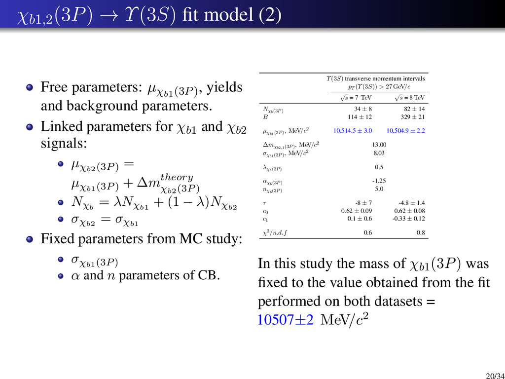
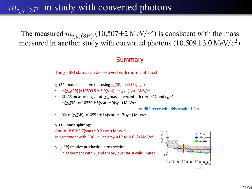
21. mχb1 (3P) in study with converted photons The measured mχb1(3P) (10,507±2 MeV/c2) is consistent with the mass measured in another study with converted photons (10,509±3.0 MeV/c2). Summary The b (3P) states can be resolved with more statistics! b (3P) mass measurement using b (3P) (1S)ee : • m(b1 (3P) )=10509.5  3.0(stat) +5.3 -2.9 (syst) MeV/c2 • ATLAS measured b1 and b2 mass barycenter for m=12 and r12 =1 : m(b (3P) )= 10530  5(stat)  9(syst) MeV/c2  difference with this result~ 1.3  • D0: m(b (3P) )=10551  14(stat)  17(syst) MeV/c2 b (1P) mass splitting: m12 = 18.6  0.7(stat)  0.2 (syst) MeV/c2 In agreement with PDG value: m12 =19.4 0.6 (?) MeV/c2 b1,2 (1P) relative production cross section: in agreement with c and theory but statistically limited 23/24 21/34
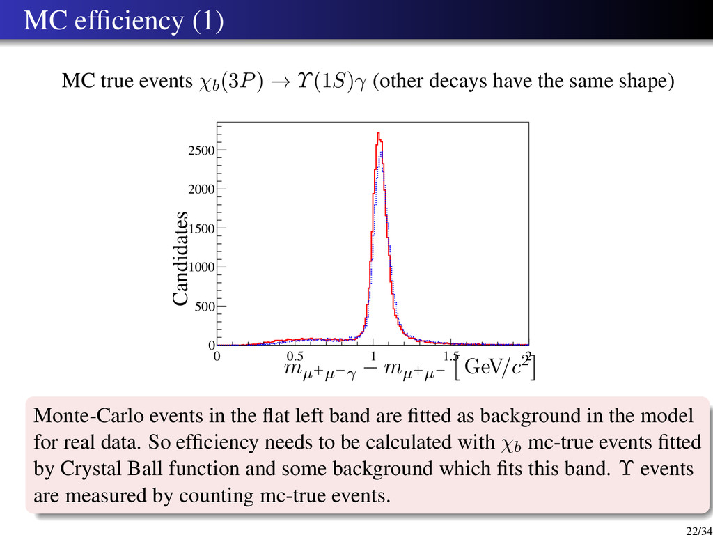
22. MC efficiency (1) MC true events χb(3P) → Υ(1S)γ (other decays have the same shape) 0 0.5 1 1.5 2 0 500 1000 1500 2000 2500 Candidates mµ+µ−γ − mµ+µ− GeV/c2 Monte-Carlo events in the flat left band are fitted as background in the model for real data. So efficiency needs to be calculated with χb mc-true events fitted by Crystal Ball function and some background which fits this band. Υ events are measured by counting mc-true events. 22/34
23. Monte-Carlo photon reconstruction (2) Example of fits: 9.8 9.9 10 10.1 0 1000 2000 3000 4000 5000 6000 -4 -2 0 2 4 χb1(1P) → Υ(1S)γ 6 < pΥ (1S) T < 40 GeV/c mµ+µ−γ − mµ+µ− + 9.4603 GeV/c2 Candidates/(10 MeV/c2) N = 34,330 ± 220 B = 5240 ± 140 (13.3 ± 0.4%) 10 10.2 10.4 10.6 0 500 1000 1500 2000 2500 -4 -2 0 2 4 χb1(2P) → Υ(1S)γ 6 < pΥ (1S) T < 40 GeV/c mµ+µ−γ − mµ+µ− + 9.4603 GeV/c2 Candidates/(10 MeV/c2) N = 22,210 ± 170 B = 2290 ± 90 (9.3 ± 0.4%) 10.2 10.4 10.6 10.8 0 200 400 600 800 1000 1200 1400 -4 -2 0 2 4 χb1(3P) → Υ(1S)γ 6 < pΥ (1S) T < 40 GeV/c mµ+µ−γ − mµ+µ− + 9.4603 GeV/c2 Candidates/(10 MeV/c2) N = 15,110 ± 130 B = 1360 ± 60 (8.26 ± 0.35%) 10.2 10.25 10.3 0 10 20 30 40 50 -4 -2 0 2 4 χb1(2P) → Υ(2S)γ 18 < pΥ (1S) T < 40 GeV/c mµ+µ−γ − mµ+µ− + 10.02326 GeV/c2 Candidates/(10 MeV/c2) N = 194 ± 21 B = 15 ± 17 (7 ± 8%) 10.4 10.5 10.6 0 20 40 60 80 100 120 -4 -2 0 2 4 χb1(3P) → Υ(2S)γ 18 < pΥ (1S) T < 40 GeV/c mµ+µ−γ − mµ+µ− + 10.02326 GeV/c2 Candidates/(10 MeV/c2) N = 672 ± 32 B = 57 ± 21 (7.8 ± 2.9%) 10.45 10.5 10.55 10.6 10.65 0 10 20 30 40 50 60 70 80 -4 -2 0 2 4 χb1(3P) → Υ(3S)γ 27 < pΥ (1S) T < 40 GeV/c mµ+µ−γ − mµ+µ− + 10.355 GeV/c2 Candidates/(10 MeV/c2) N = 154 ± 17 B = 113 ± 16 (42 ± 7%) 23/34
24. Data — Monte Carlo comparison A comparison of the distribution of the relevant observables used in this analysis was performed on real and simulated data, in order to assess the reliability of Monte Carlo in computing efficiencies 0 0.2 0.4 0.6 0.8 1 0 0.01 0.02 0.03 0.04 0.05 0.06 0 0.2 0.4 0.6 0.8 1 0 0.01 0.02 0.03 0.04 0.05 0.06 0 0.2 0.4 0.6 0.8 1 -0.02 0 0.02 0.04 0.06 0.08 0.1 0 2 4 0 0.01 0.02 0.03 0.04 0.05 0.06 0.07 0.08 0 2 4 0 0.02 0.04 0.06 0.08 0 2 4 -0.02 0 0.02 0.04 0.06 0.08 0.1 0.12 0.14 0 10 20 30 0 0.01 0.02 0.03 0.04 0.05 0.06 0.07 0.08 0 10 20 30 0 0.02 0.04 0.06 0.08 0.1 0 10 20 30 -0.02 0 0.02 0.04 0.06 0.08 0.1 0.12 0.14 0.16 15 20 25 30 35 0 0.01 0.02 0.03 0.04 0.05 0.06 15 20 25 30 35 0 0.02 0.04 0.06 0.08 0.1 15 20 25 30 35 0 0.05 0.1 0.15 0.2 γ confidence level γ confidence level γ confidence level χ2 of decay tree fitter χ2 of decay tree fitter χ2 of decay tree fitter pT [χb(1P)] GeV/c2 pT [χb(2P)] GeV/c2 pT [χb(3P)] GeV/c2 pT [Υ(1S)] GeV/c2 pT [Υ(1S)] GeV/c2 pT [Υ(1S)] GeV/c2 Arbitrary units Arbitrary units Arbitrary units Arbitrary units Arbitrary units Arbitrary units Arbitrary units Arbitrary units Arbitrary units Arbitrary units Arbitrary units Arbitrary units χb(1P) χb(2P) χb(3P) χb(1P) χb(2P) χb(3P) χb(1P) χb(2P) χb(3P) χb(1P) χb(2P) χb(3P) The agreement is generally very good. 24/34
25. Monte-Carlo photon reconstruction efficiency χb(1P), χb(2P), χb(3P) reconstruction efficiency in χb → Υγ decays. 10 15 20 25 30 0 5 10 15 20 25 30 35 20 25 30 35 40 0 5 10 15 20 25 30 35 Efficiency (%) pT (Υ(1S)) GeV/c2 χb(1, 2, 3P ) → Υ (1S)γ Efficiency (%) pT (Υ(2S)) GeV/c2 χb(2, 3P ) → Υ (2S)γ Photons is more energetic as pT (Υ) increases so it is reconstructed more efficiently. 25/34
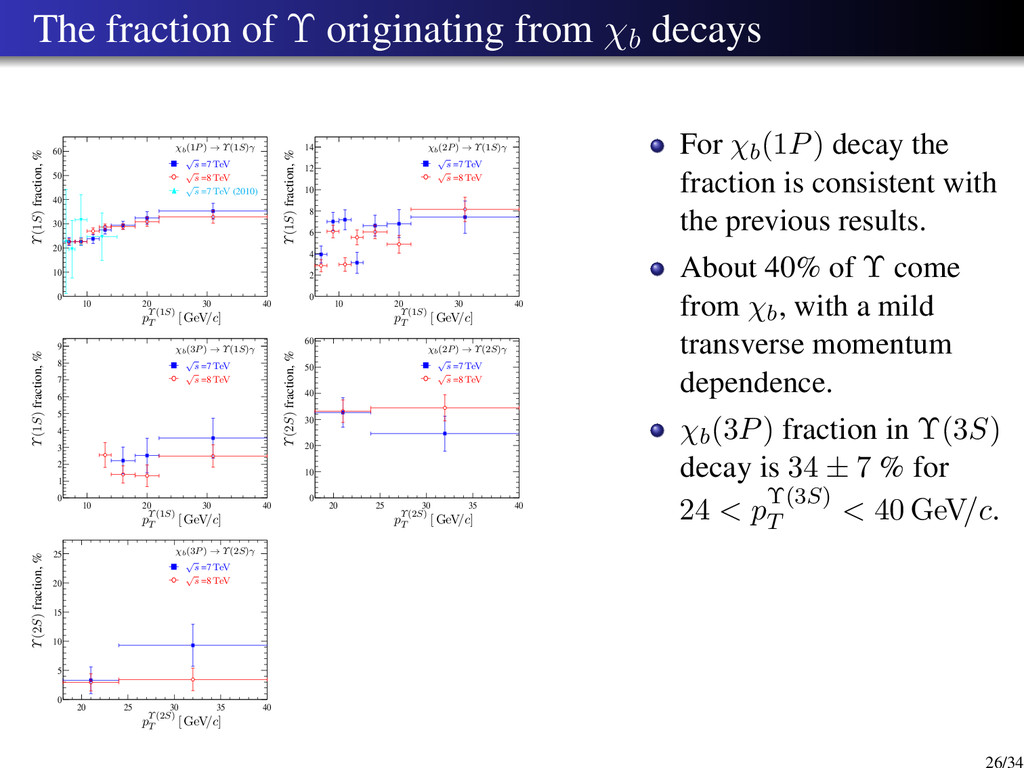
26. The fraction of Υ originating from χb decays 10 20 30 40 0 10 20 30 40 50 60 Υ(1S) fraction, % pΥ(1S) T [ GeV/c] χb(1P) → Υ(1S)γ √ s =7 TeV √ s =8 TeV √ s =7 TeV (2010) 10 20 30 40 0 2 4 6 8 10 12 14 Υ(1S) fraction, % pΥ(1S) T [ GeV/c] χb(2P) → Υ(1S)γ √ s =7 TeV √ s =8 TeV 10 20 30 40 0 1 2 3 4 5 6 7 8 9 Υ(1S) fraction, % pΥ(1S) T [ GeV/c] χb(3P) → Υ(1S)γ √ s =7 TeV √ s =8 TeV 20 25 30 35 40 0 10 20 30 40 50 60 Υ(2S) fraction, % pΥ(2S) T [ GeV/c] χb(2P) → Υ(2S)γ √ s =7 TeV √ s =8 TeV 20 25 30 35 40 0 5 10 15 20 25 Υ(2S) fraction, % pΥ(2S) T [ GeV/c] χb(3P) → Υ(2S)γ √ s =7 TeV √ s =8 TeV For χb(1P) decay the fraction is consistent with the previous results. About 40% of Υ come from χb, with a mild transverse momentum dependence. χb(3P) fraction in Υ(3S) decay is 34 ± 7 % for 24 < pΥ(3S) T < 40 GeV/c. 26/34
27. Systematic uncertainties due to λ = Nχb1 /(Nχb1 + Nχb2 ) ratio in χb (1, 2, 3P) → Υ(1S)γ decays Υ(1S) transverse momentum intervals 6 < pT < 8 GeV/c 8 < pT < 10 GeV/c 10 < pT < 12 GeV/c 12 < pT < 14 GeV/c λ / Change (%) Nχb(1P) Nχb(2P) Nχb(3P) Nχb(1P) Nχb(2P) Nχb(3P) Nχb(1P) Nχb(2P) Nχb(3P) Nχb(1P) Nχb(2P) Nχb(3P) 0.0 19 -9 - 24 -3 - 24 -20 - 16 -1 -6 0.1 13 -8 - 18 -3 - 18 -17 - 12 -2 -4 0.2 8 -5 - 12 -2 - 12 -13 - 8 -2 -2 0.3 4 -4 - 7 -2 - 7 -9 - 5 -2 -1 0.4 2 -3 - 3 -1 - 3 -5 - 2 -2 0 0.5 0 -2 - 0 0 - 1 -3 - 1 -1 1 0.6 0 1 - -1 1 - 0 0 - 0 0 1 0.7 1 -1 - -1 1 - 0 1 - 0 2 0 0.8 3 -2 - 0 1 - 2 2 - 1 4 0 0.9 7 -5 - 3 1 - 5 1 - 3 6 -1 1.0 10 -9 - 6 1 - 9 0 - 5 9 -2 Υ(1S) transverse momentum intervals 14 < pT < 18 GeV/c 18 < pT < 22 GeV/c 22 < pT < 30 GeV/c 18 < pT < 30 GeV/c λ / Change (%) Nχb(1P) Nχb(2P) Nχb(3P) Nχb(1P) Nχb(2P) Nχb(3P) Nχb(1P) Nχb(2P) Nχb(3P) Nχb(1P) Nχb(2P) Nχb(3P) 0.0 15 1 -14 12 0 -5 9 -5 -11 11 -2 -8 0.1 11 0 -10 8 -1 -3 6 -4 -9 7 -2 -5 0.2 7 0 -6 5 -1 -1 3 -4 -6 4 -2 -3 0.3 4 -1 -3 2 -1 0 1 -3 -4 2 -2 -1 0.4 2 -1 -1 1 -1 0 0 -2 -3 0 -1 0 0.5 0 -1 1 0 -1 0 -1 -1 -1 0 0 1 0.6 0 0 1 0 0 0 0 0 0 0 0 1 0.7 1 0 1 1 1 -1 1 1 1 1 1 1 0.8 2 2 0 2 2 -3 4 2 2 3 3 0 0.9 4 3 -1 5 4 -3 7 3 2 6 5 0 1.0 7 5 -2 8 7 -4 10 5 3 9 7 0 Theory predicts lambda in range [0.4,0.6]. When varying lambda in this range, the maximum uncertainty on the yields is 4%, 5% and 3% for Nχb(1P), Nχb(2P) and Nχb(3P), respectively. 27/34
28. Systematic uncertainties due to λ = Nχb1 /(Nχb1 + Nχb2 ) ratio in χb (2, 3P) → Υ(2S)γ decays Υ(2S) transverse momentum intervals 18 < pT < 25 GeV/c 25 < pT < 40 GeV/c λ / Change (%) Nχb(2P) Nχb(3P) Nχb(2P) Nχb(3P) 0.0 12 10 12 -4 0.1 7 6 8 -3 0.2 4 3 6 -7 0.3 1 1 3 -5 0.4 0 0 1 -3 0.5 0 0 0 0 0.6 1 1 -2 11 0.7 4 4 1 8 0.8 7 8 3 12 0.9 11 13 6 17 1.0 17 19 10 22 Theory predicts lambda in range [0.4,0.6]. When varying lambda in this range, the maximum uncertainty on the yields is 2% and 11% for Nχb(2P) and Nχb(3P), respectively. 28/34
29. Systematic uncertainties due to mχb1 (1P) mass range in χb (1, 2, 3P) → Υ(1S)γ decays. Uncertainty due to the χb1(1P) mass variation in the pΥ(1S) T range is estimated by using the observed minimum and maximum values. Υ(1S) transverse momentum intervals 6 < pT < 8 GeV/c 8 < pT < 10 GeV/c 10 < pT < 12 GeV/c 12 < pT < 14 GeV/c m(χb1(1P)) / Change (%) Nχb(1P) Nχb(2P) Nχb(3P) Nχb(1P) Nχb(2P) Nχb(3P) Nχb(1P) Nχb(2P) Nχb(3P) Nχb(1P) Nχb(2P) Nχb(3P) 9.885 GeV/c2 (min [m(χb1(1P))]) -1 0 - -6 2 - 0 5 - -2 6 1 9.896 GeV/c2 (max [m(χb1(1P))]) 4 -1 - 6 -1 - 4 -5 - 3 -2 -1 Υ(1S) transverse momentum intervals 14 < pT < 18 GeV/c 18 < pT < 22 GeV/c 22 < pT < 30 GeV/c 18 < pT < 30 GeV/c m(χb1(1P)) / Change (%) Nχb(1P) Nχb(2P) Nχb(3P) Nχb(1P) Nχb(2P) Nχb(3P) Nχb(1P) Nχb(2P) Nχb(3P) Nχb(1P) Nχb(2P) Nχb(3P) 9.885 GeV/c2 (min [m(χb1(1P))]) -1 2 4 1 4 -2 3 5 8 2 5 2 9.896 GeV/c2 (max [m(χb1(1P))]) 2 0 -3 1 0 1 0 -2 -5 1 -2 -2 Maximum uncertainty on the yields is 6%, 6% and 8% for Nχb(1P), Nχb(2P) and Nχb(3P), respectively. 29/34
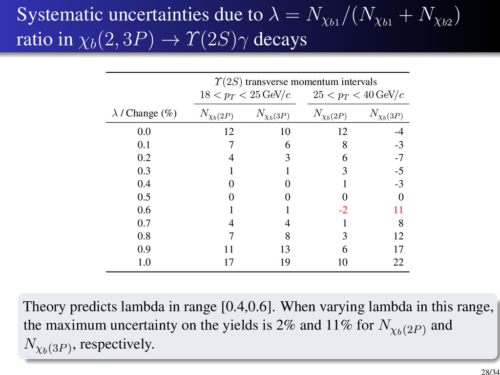
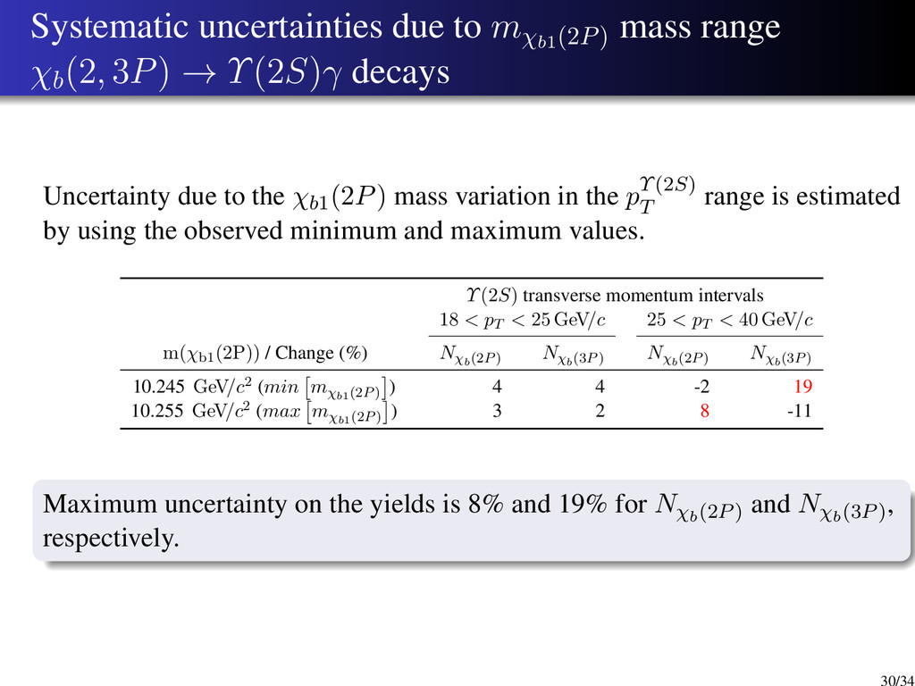
30. Systematic uncertainties due to mχb1 (2P) mass range χb (2, 3P) → Υ(2S)γ decays Uncertainty due to the χb1(2P) mass variation in the pΥ(2S) T range is estimated by using the observed minimum and maximum values. Υ(2S) transverse momentum intervals 18 < pT < 25 GeV/c 25 < pT < 40 GeV/c m(χb1(2P)) / Change (%) Nχb(2P) Nχb(3P) Nχb(2P) Nχb(3P) 10.245 GeV/c2 (min mχb1(2P) ) 4 4 -2 19 10.255 GeV/c2 (max mχb1(2P) ) 3 2 8 -11 Maximum uncertainty on the yields is 8% and 19% for Nχb(2P) and Nχb(3P), respectively. 30/34
31. Systematic uncertainties due to mχb1 (3P) mass range in χb (1, 2, 3P) → Υ(1S)γ and χb (2, 3P) → Υ(2S)γ decays Uncertainty due to the χb1(3P) mass variation in the pΥ T range is estimated by using the observed minimum and maximum values. Υ(1S) transverse momentum intervals 14 < pT < 18 GeV/c 18 < pT < 22 GeV/c 22 < pT < 30 GeV/c 18 < pT < 30 GeV/c m(χb1(3P)) / Change (%) Nχb(1P) Nχb(2P) Nχb(3P) Nχb(1P) Nχb(2P) Nχb(3P) Nχb(1P) Nχb(2P) Nχb(3P) Nχb(1P) Nχb(2P) Nχb(3P) 10.503 GeV/c2 (min [m(χb1(3P))]) 0 -1 -6 0 1 7 0 0 1 0 1 5 10.517 GeV/c2 (max [m(χb1(3P))]) 0 3 19 0 -2 -14 0 0 -2 0 -1 -9 Maximum uncertainty on the yields is 3% and 19% for Nχb(2P) an Nχb(3P), respectively. Υ(2S) transverse momentum intervals 18 < pT < 25 GeV/c 25 < pT < 40 GeV/c m(χb1(3P)) / Change (%) Nχb(2P) Nχb(3P) Nχb(2P) Nχb(3P) 10.503 GeV/c2 (min [m(χb1(3P))]) 0 -1 0 -4 10.517 GeV/c2 (max [m(χb1(3P))]) 0 4 0 -8 Maximum uncertainty on the yields is 8% for Nχb(3P). 31/34
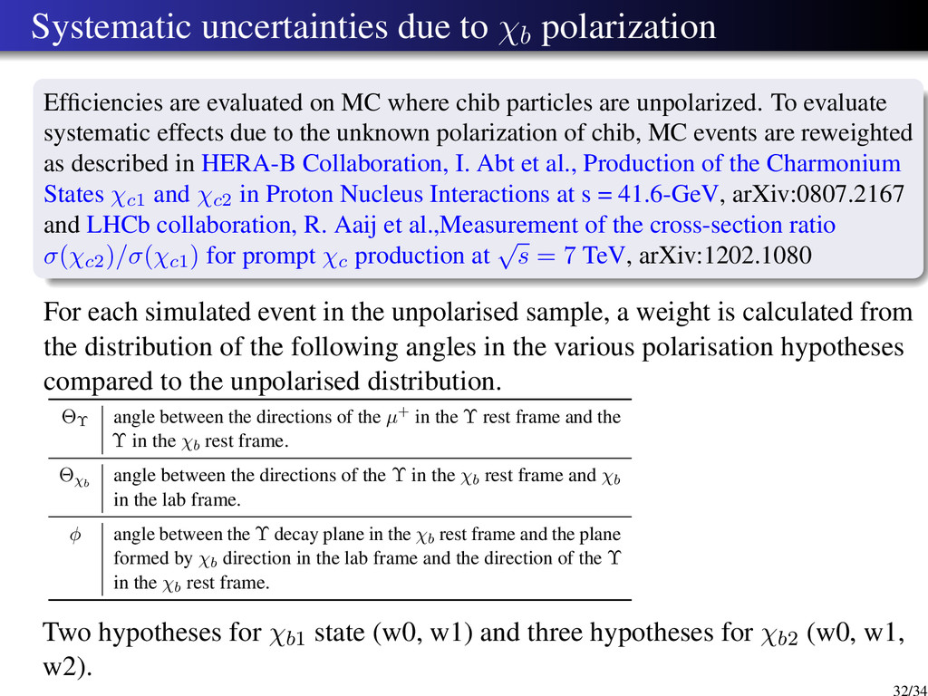
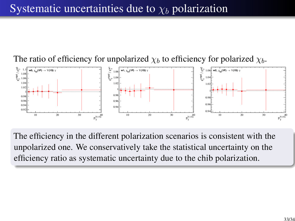
32. Systematic uncertainties due to χb polarization Efficiencies are evaluated on MC where chib particles are unpolarized. To evaluate systematic effects due to the unknown polarization of chib, MC events are reweighted as described in HERA-B Collaboration, I. Abt et al., Production of the Charmonium States χc1 and χc2 in Proton Nucleus Interactions at s = 41.6-GeV, arXiv:0807.2167 and LHCb collaboration, R. Aaij et al.,Measurement of the cross-section ratio σ(χc2 )/σ(χc1 ) for prompt χc production at √ s = 7 TeV, arXiv:1202.1080 For each simulated event in the unpolarised sample, a weight is calculated from the distribution of the following angles in the various polarisation hypotheses compared to the unpolarised distribution. ΘΥ angle between the directions of the µ+ in the Υ rest frame and the Υ in the χb rest frame. Θχb angle between the directions of the Υ in the χb rest frame and χb in the lab frame. φ angle between the Υ decay plane in the χb rest frame and the plane formed by χb direction in the lab frame and the direction of the Υ in the χb rest frame. Two hypotheses for χb1 state (w0, w1) and three hypotheses for χb2 (w0, w1, w2). 32/34
33. Systematic uncertainties due to χb polarization The ratio of efficiency for unpolarized χb to efficiency for polarized χb. (1S) Υ T p 10 20 30 40 w0 γ ε / unpol γ ε 0.92 0.94 0.96 0.98 1 1.02 1.04 1.06 1.08 1.1 γ (1S) Υ → (1P) b2 χ w0, γ (1S) Υ → (1P) b2 χ w0, (1S) Υ T p 10 20 30 40 w1 γ ε / unpol γ ε 0.94 0.96 0.98 1 1.02 1.04 1.06 γ (1S) Υ → (1P) b2 χ w1, γ (1S) Υ → (1P) b2 χ w1, (1S) Υ T p 10 20 30 40 w2 γ ε / unpol γ ε 0.94 0.96 0.98 1 1.02 1.04 1.06 γ (1S) Υ → (1P) b2 χ w2, γ (1S) Υ → (1P) b2 χ w2, The efficiency in the different polarization scenarios is consistent with the unpolarized one. We conservatively take the statistical uncertainty on the efficiency ratio as systematic uncertainty due to the chib polarization. 33/34
34. Summary Measured fractions of Υ(1, 2, 3S) originated from χb decays. About 40% of Υ come from χb, with mild dependence on Υ transverse momentum. Measured mass of χb(3P) is 10507±2 MeV/c2, consistent with another determination which uses converted photons. An LHCb internal note documenting this study has been written. The analysis is currently under internal review and will be the subject of an LHCb publication. 34/34