Smart Algorithms for Smart Grids

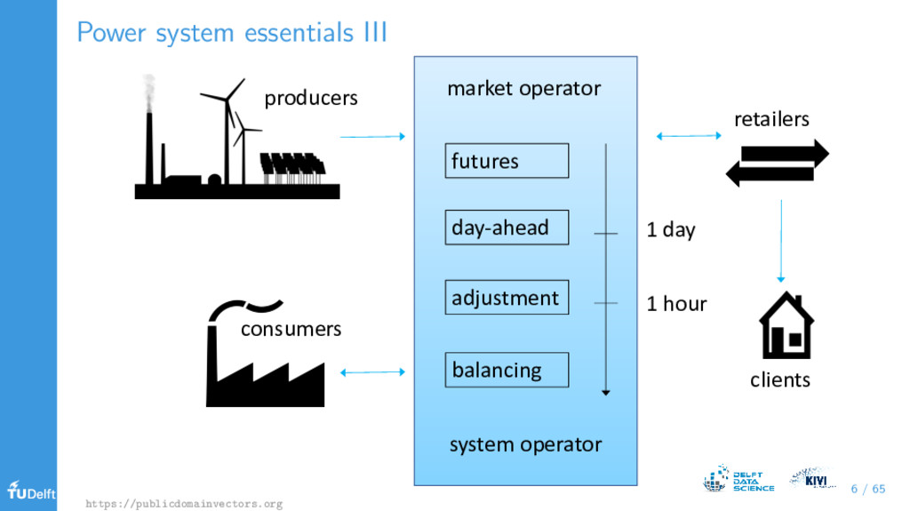
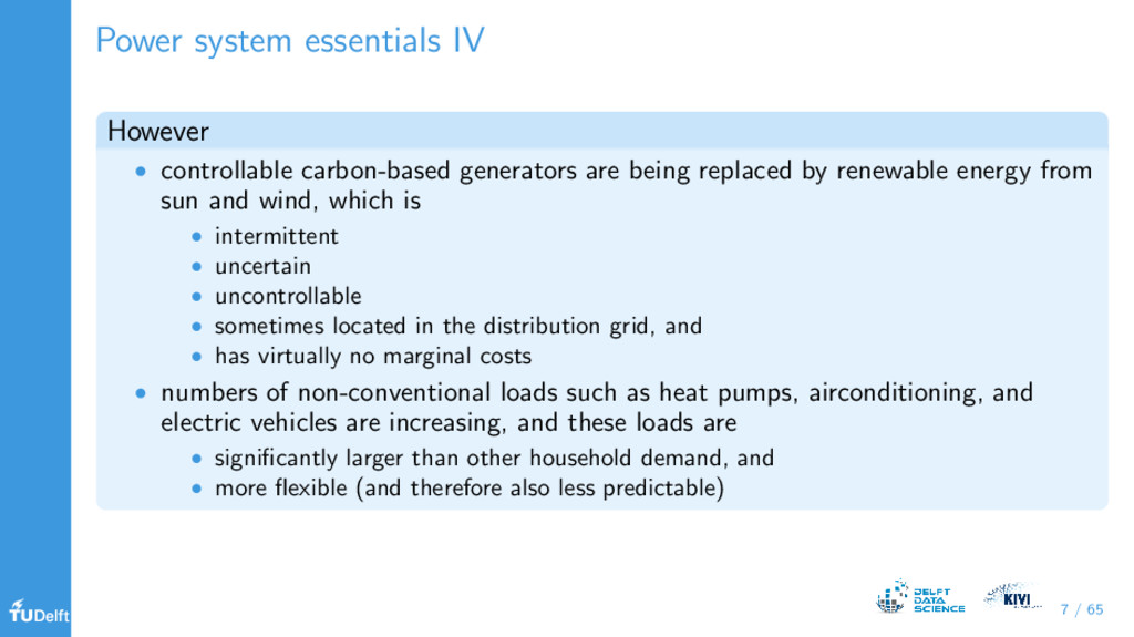
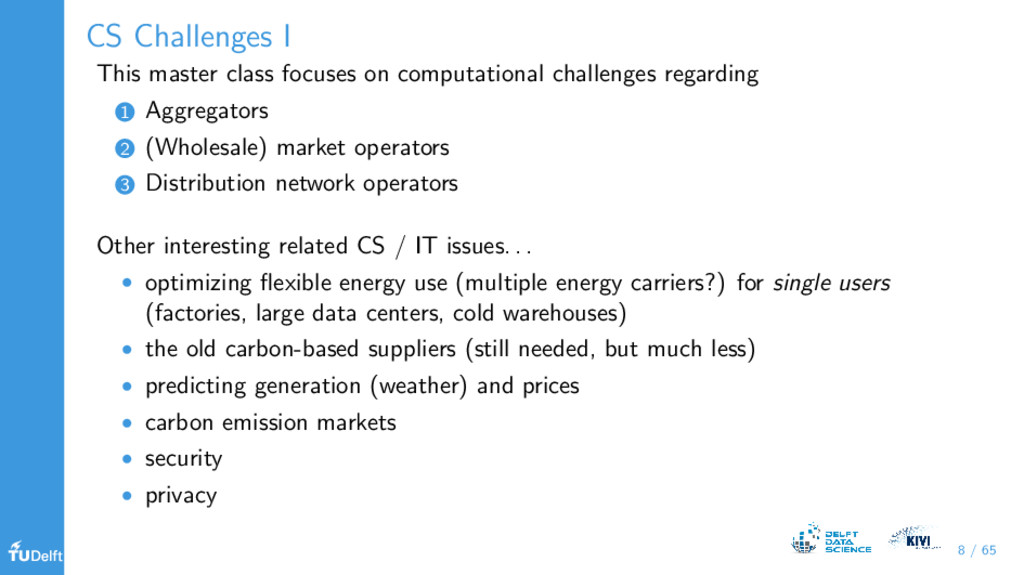
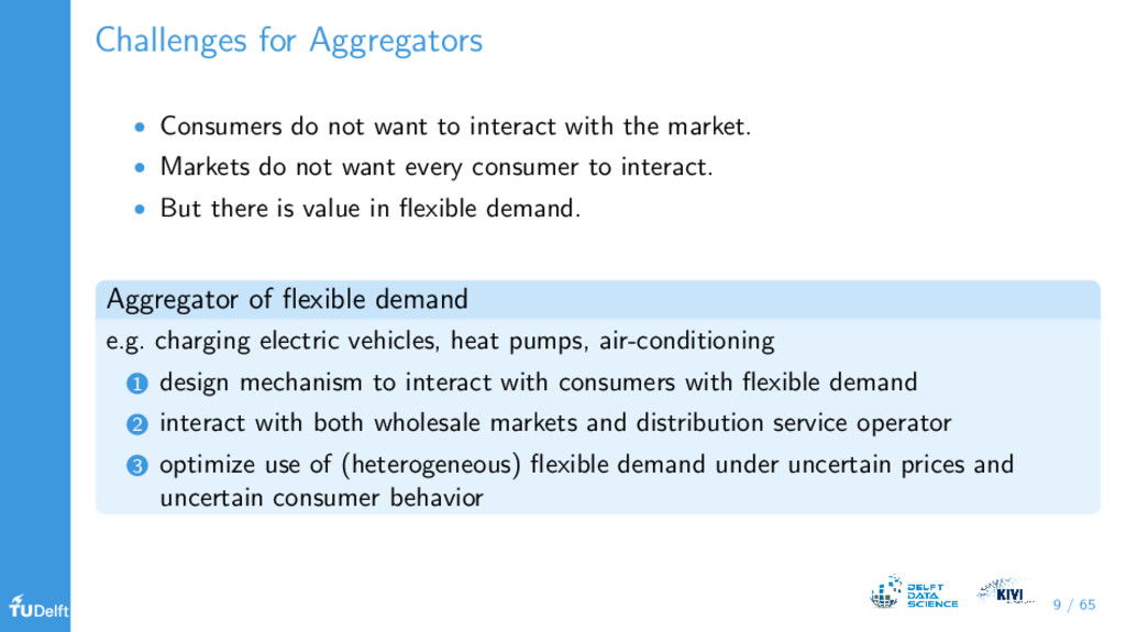
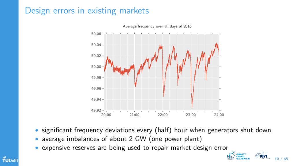
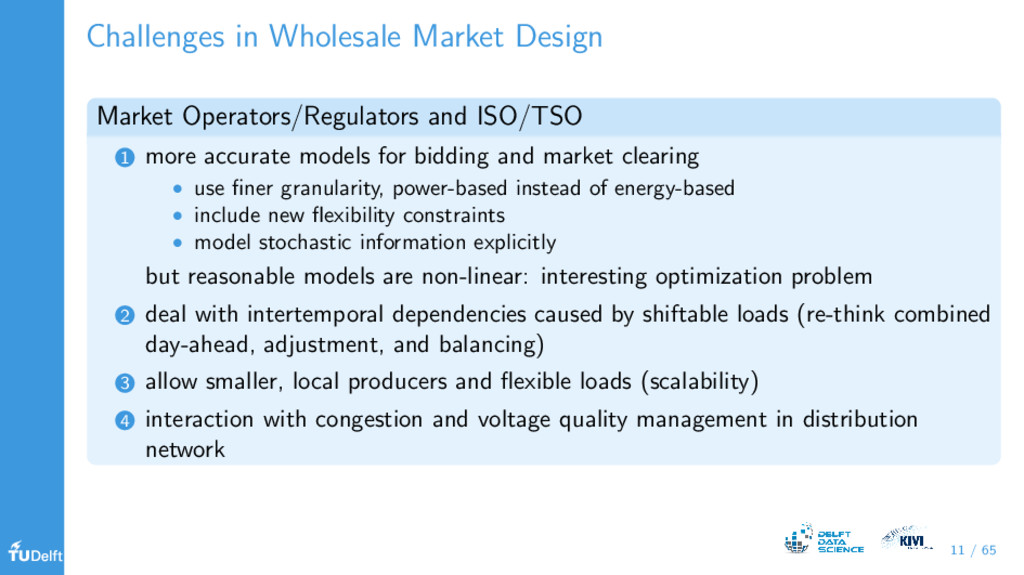
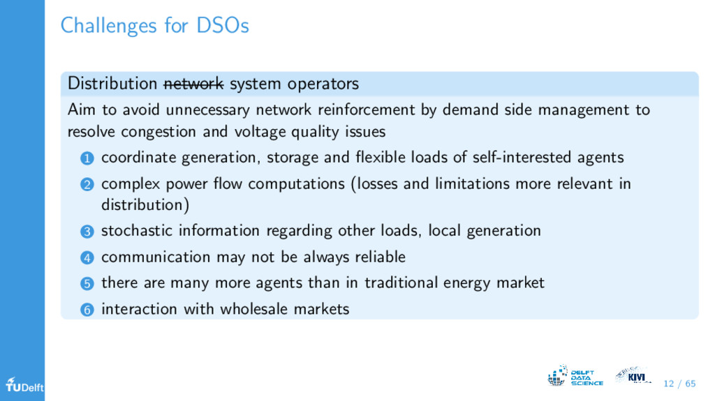
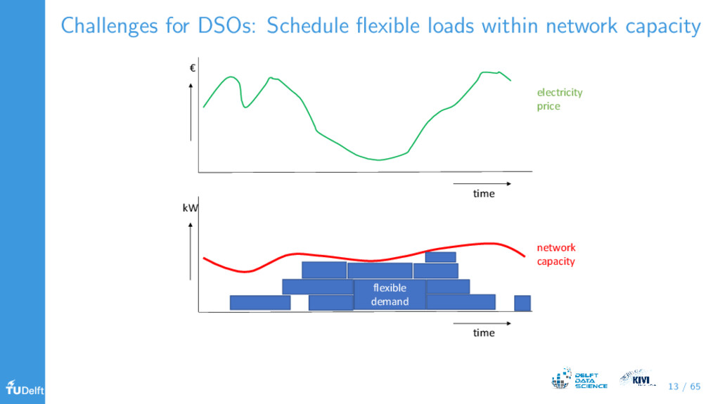
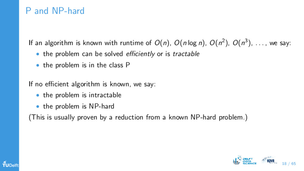
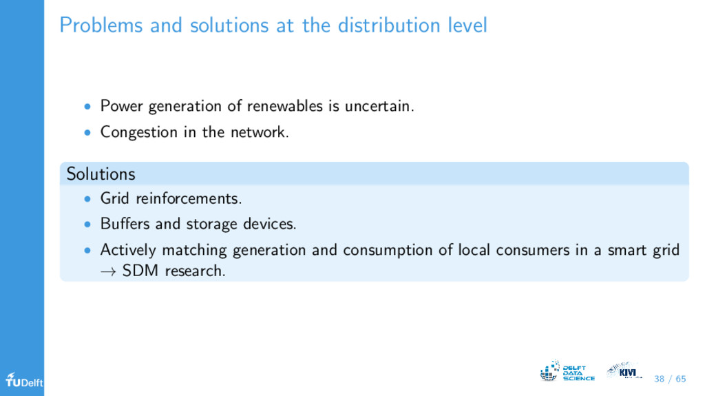
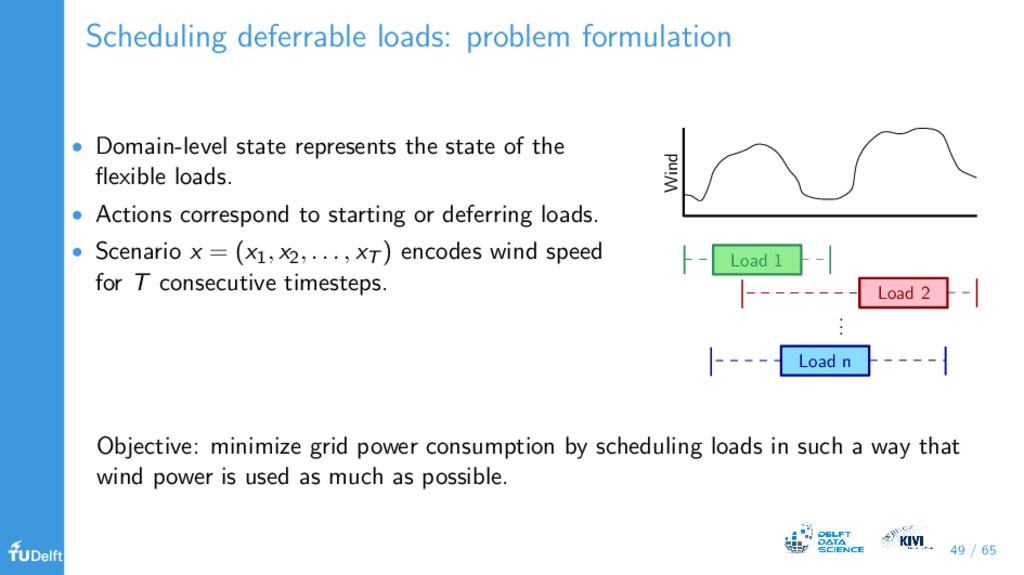
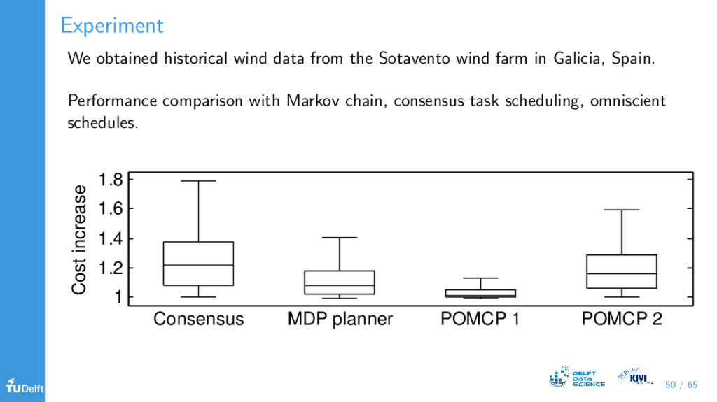
A domain with an enormous potential for planning algorithms is the smart grid. Renewables and flexible demand such as heat pumps and charging of electric vehicles bring more uncertainty, and also computational challenges for several parties in the electricity sector. There is the new role of an aggregator to schedule and trade the flexibility of demand in the electricity markets. The electricity markets themselves may need to be redesigned because of the intermittency of generation and flexible demand, resulting in more complexity in clearing the market. Distribution network operators need to coordinate the flexible demand in congested areas to prevent more demand shifting to a moment in time (with the lowest electricity price) than the capacity of the network allows. Each of these new challenges in the smart grid gives rise to an interesting optimization problem. Interesting, because typically they are NP-hard: there is no known algorithm that can directly solve such realistically-sized problems quickly enough.

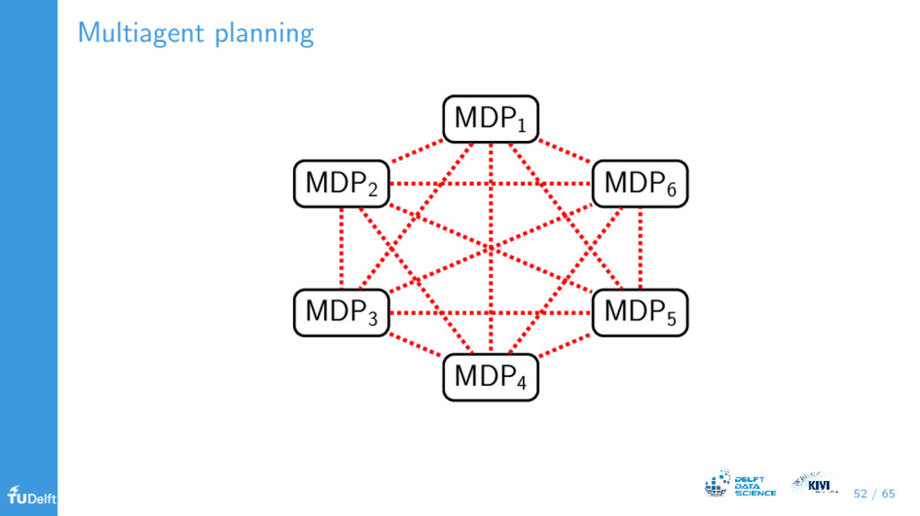
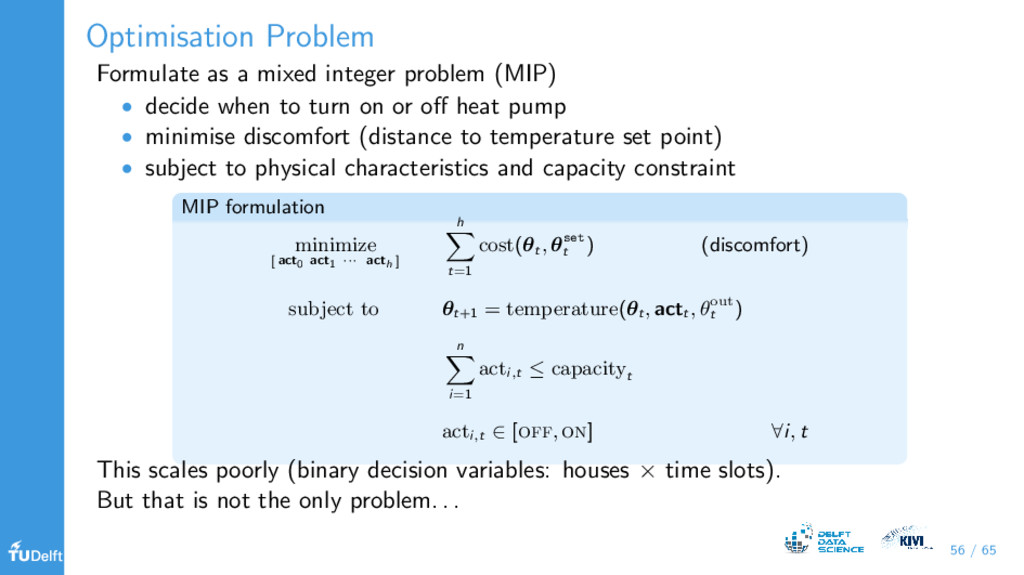
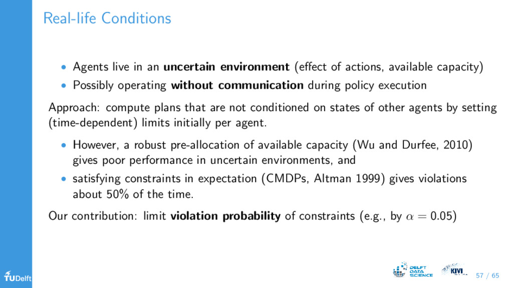
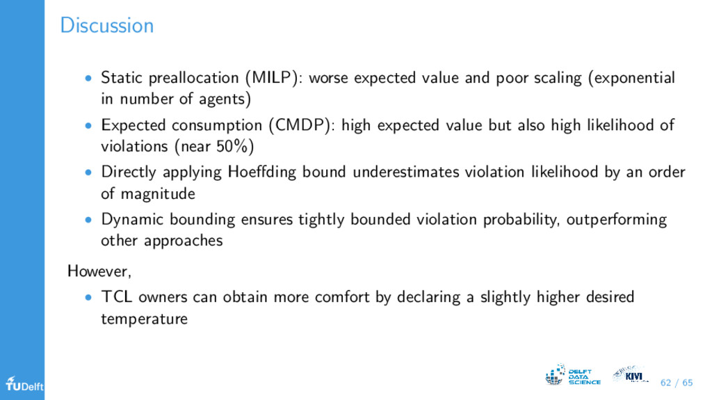
In our research we tackle such challenges by identifying and exploiting some structure in these problems. For example, to schedule a large number of heat pumps under a single network capacity constraint, we decouple the scheduling problems for the individual heat pumps as much as possible by representing the value for the network capacity of all heat pumps by an artificial `price’ for each moment in time. See also this blog post on the recently accepted paper by Frits de Nijs for the case where the constraint is not exactly known in advance (because of non-flexible demand on the network).

Transcript

1. Smart Algorithms for Smart Grids dr. Mathijs de Weerdt & dr. Matthijs Spaan
2. Main message The energy system is changing. The future energy system is a rich environment with many challenges for computer scientists. 2 / 65
3. Overview 1 First example: EV charging 2 Power System Essentials for non-Electrical Engineers 3 CS Challenges in the Future Power Grid 4 (10 minute break) 5 Techniques for Decision Making 6 Concrete Examples of Smart Algorithms for Smart Grids 1 Decision making with wind scenarios (Walraven & Spaan, 2015) 2 Planning and coordination of thermostatic loads (de Nijs et al., 2015, 2017) 7 Discussion 3 / 65
4. Power system essentials I • Most significant changes are in the electricity systems. • Electricity systems support the generation, transport and use of electrical energy. • They are large and complex. Energy generated = energy consumed at all times How it used to be. . . • demand is predictable (at an aggregate level, day ahead) • which generators are used is decided one day in advance (unit commitment), taking into account transmission constraints • a market with 2–10 actors (energy retailers) • minor corrections are made, based on frequency (primary control, secondary control, etc.) 4 / 65
5. Power system essentials II Electrical grid design Specifically for this mode of operation (50–100 years ago): • transmission at high voltage to transport large amounts over long distances (thick cables, little losses, redundancy, few nodes), actively measured and controlled, • distribution to bring energy to the end-users (thinner cables, lower voltages, safer, cheaper, but higher losses, star topology, many nodes), passively operated, • over-dimensioned: designed for peak demand (Christmas day) 5 / 65
6. Power system essentials III market operator system operator futures day-ahead adjustment balancing 1 day 1 hour producers consumers retailers clients https://publicdomainvectors.org 6 / 65
7. Power system essentials IV However • controllable carbon-based generators are being replaced by renewable energy from sun and wind, which is • intermittent • uncertain • uncontrollable • sometimes located in the distribution grid, and • has virtually no marginal costs • numbers of non-conventional loads such as heat pumps, airconditioning, and electric vehicles are increasing, and these loads are • significantly larger than other household demand, and • more flexible (and therefore also less predictable) 7 / 65
8. CS Challenges I This master class focuses on computational challenges regarding 1 Aggregators 2 (Wholesale) market operators 3 Distribution network operators Other interesting related CS / IT issues. . . • optimizing flexible energy use (multiple energy carriers?) for single users (factories, large data centers, cold warehouses) • the old carbon-based suppliers (still needed, but much less) • predicting generation (weather) and prices • carbon emission markets • security • privacy 8 / 65
9. Challenges for Aggregators • Consumers do not want to interact with the market. • Markets do not want every consumer to interact. • But there is value in flexible demand. Aggregator of flexible demand e.g. charging electric vehicles, heat pumps, air-conditioning 1 design mechanism to interact with consumers with flexible demand 2 interact with both wholesale markets and distribution service operator 3 optimize use of (heterogeneous) flexible demand under uncertain prices and uncertain consumer behavior 9 / 65
10. Design errors in existing markets Average frequency over all days of 2016 20:00 21:00 22:00 23:00 24:00 1 49.92 49.94 49.96 49.98 50.00 50.02 50.04 50.06 • significant frequency deviations every (half) hour when generators shut down • average imbalances of about 2 GW (one power plant) • expensive reserves are being used to repair market design error 10 / 65
11. Challenges in Wholesale Market Design Market Operators/Regulators and ISO/TSO 1 more accurate models for bidding and market clearing • use finer granularity, power-based instead of energy-based • include new flexibility constraints • model stochastic information explicitly but reasonable models are non-linear: interesting optimization problem 2 deal with intertemporal dependencies caused by shiftable loads (re-think combined day-ahead, adjustment, and balancing) 3 allow smaller, local producers and flexible loads (scalability) 4 interaction with congestion and voltage quality management in distribution network 11 / 65
12. Challenges for DSOs Distribution network system operators Aim to avoid unnecessary network reinforcement by demand side management to resolve congestion and voltage quality issues 1 coordinate generation, storage and flexible loads of self-interested agents 2 complex power flow computations (losses and limitations more relevant in distribution) 3 stochastic information regarding other loads, local generation 4 communication may not be always reliable 5 there are many more agents than in traditional energy market 6 interaction with wholesale markets 12 / 65
13. Challenges for DSOs: Schedule flexible loads within network capacity time flexible demand electricity price network capacity time € kW 13 / 65
14. Computational Limitations: Complexity Theory Sometimes problems are easy. Example problem: Scheduling to minimize the maximum lateness • Given a set of n jobs with for each job j length pj and deadline dj • Schedule all of them such that the maximum lateness over jobs is minimized. • The lateness of a job is max{0, dj − fj }, where fj is the finish time of a job in the schedule. 14 / 65
15. Scheduling to Minimize Maximum Lateness Algorithm pseudocode Sort jobs by deadline so that d1 ≤ d2 ≤ . . . ≤ dn t ← 0 for j ← 1, 2, . . . , n do sj ← t // Assign job j to interval [t, t + pj ] fj ← t + pj t ← fj Output intervals [sj , fj ] The runtime consists of sorting: O(n log n) and then n steps in the for-loop. 15 / 65
16. Runtime complexity 16 / 65
17. Runtime complexity (log scale) 17 / 65
18. P and NP-hard If an algorithm is known with runtime of O(n), O(n log n), O(n2), O(n3), . . . , we say: • the problem can be solved efficiently or is tractable • the problem is in the class P If no efficient algorithm is known, we say: • the problem is intractable • the problem is NP-hard (This is usually proven by a reduction from a known NP-hard problem.) 18 / 65
19. Example of a known NP-hard problem Traveling salesman problem • What is the most efficient route to arrange a school bus route to pick-up children? • What is the most efficient order for a machine to drill holes holes in a circuit board? Given • n cities with distances d(i, j) • Find the shortest path from city 1 through all cities back to 1 19 / 65
20. Consequence of NP-hardness We must sacrifice one of three desired features. 1 We cannot solve problem in polynomial time. 2 We cannot solve problem to optimality. 3 We cannot solve arbitrary instances of the problem. 20 / 65
21. Example: Complexity of Charging EVs in Constrained Smart Grid Mathijs de Weerdt, Michael Alberts, and Vincent Conitzer (Duke University) Results: • equivalence to single-machine scheduling variants if charging speeds are identical • hardness results if vehicles not always available (“gaps”) or with complex demand/charging speeds • dynamic programs for constant horizon problems 21 / 65
22. Dynamic Programming Main idea: divide into subproblems, reuse solutions from subproblems • Characterize structure of problem • Recursively define value of optimal solution: OPT(i) = . . . • Compute value of optimal solution iteratively starting from smallest • Construct optimal solution from computed information 22 / 65
23. Dynamic Programming for Charging EVs • |T| periods, n agents • supply per period t ∈ T of mt ≤ M • demand per agent at most L encoded in constraints on possible allocation a • vi (a) denotes value for agent i for allocation a Optimal solution OPT(m1, m2, . . . , m|T| , n) computed using: OPT(m1 , m2 , . . . , m|T| , i) = 0 if i = 0 max OPT(m1 , m2 , . . . , m|T| , i − 1), o otherwise where o = max a1,.,a|T| OPT(m1 − a1 , . . . , m|T| − a|T| , i − 1) + vi (a) . Runtime of dynamic programming implemenation: O n · M|T| · L|T| 23 / 65
24. Example: Complexity of Charging EVs in Constrained Smart Grid Typical scenario: constraint in substation for 20–500, prices that differ per 15 minute Conclusions: • Scheduling of about 20 electric vehicles in a rolling horizon setting of 1.5 hours doable, but • more than 10% EVs or look-ahead more than 1.5 hours, we need to sacrifice optimality. • Without bounds on infrastructure or on charging speed, realistically-sized problems can be solved quickly. 24 / 65
25. Techniques for Decision Making • Efficient algorithms: greedy, dynamic programming • Approaches to NP-hard problems: integer programming, planning and multi-agent planning • Concrete examples 25 / 65
26. Integer Programming z = max x,y 16x + 10y s.t. x + y ≤ 11.5 4x + 2y ≤ 33 x, y ≥ 0 x, y ∈ R + Simplex Method (1947): 26 / 65
27. Introduction to planning in Artificial Intelligence • Goal in Artificial Intelligence: to build intelligent agents. • Our definition of “intelligent”: perform an assigned task as well as possible. • Problem: how to act? • We will explicitly model uncertainty. 27 / 65
28. Agents • An agent is a (rational) decision maker who is able to perceive its external (physical) environment and act autonomously upon it. • Rationality means reaching the optimum of a performance measure. • Examples: humans, robots, some software programs. 28 / 65
29. Agents environment agent action observation state • It is useful to think of agents as being involved in a perception-action loop with their environment. • But how do we make the right decisions? 29 / 65
30. Planning Planning: • A plan tells an agent how to act. • For instance • A sequence of actions to reach a goal. • What to do in a particular situation. • We need to model: • the agent’s actions • its environment • its task We will model planning as a sequence of decisions. 30 / 65
31. Classic planning • Classic planning: sequence of actions from start to goal. • Task: robot should get to gold as quickly as possible. • Actions: → ↓ ← ↑ • Limitations: • New plan for each start state. • Environment is deterministic. • Three optimal plans: → → ↓, → ↓ →, ↓ → →. 31 / 65
32. Conditional planning • Assume our robot has noisy actions (wheel slip, overshoot). • We need conditional plans. • Map situations to actions. 32 / 65
33. Decision-theoretic planning 10 −0 . 1 −0 . 1 −0 . 1 −0 . 1 −0 . 1 −0 . 1 −0 . 1 −0 . 1 −0 . 1 • Positive reward when reaching goal, small penalty for all other actions. • Agent’s plan maximizes value: the sum of future rewards. • Decision-theoretic planning successfully handles noise in acting and sensing. 33 / 65
34. Decision-theoretic planning Optimal values (encode optimal plan): Reward: 10 −0 . 1 −0 . 1 −0 . 1 −0 . 1 −0 . 1 −0 . 1 −0 . 1 −0 . 1 −0 . 1 34 / 65
35. Sequential decision making under uncertainty • Uncertainty is abundant in real-world planning domains. • Bayesian approach ⇒ probabilistic models. Main assumptions: Sequential decisions: problems are formulated as a sequence of “independent” decisions; Markovian environment: the state at time t depends only on the events at time t − 1; Evaluative feedback: use of a reinforcement signal as performance measure (reinforcement learning); 35 / 65
36. Transition model • For instance, robot motion is inaccurate. • Transitions between states are stochastic. • p(s |s, a) is the probability to jump from state s to state s after taking action a. 36 / 65
37. MDP Agent environment action a obs. s reward r π state s 37 / 65
38. Problems and solutions at the distribution level • Power generation of renewables is uncertain. • Congestion in the network. Solutions • Grid reinforcements. • Buffers and storage devices. • Actively matching generation and consumption of local consumers in a smart grid → SDM research. 38 / 65
39. Why coordination and control is hard • Thousands of loads and generators connected to the grid. • Communication infrastructure might fail. • Heterogeneous characteristics and objectives. • Capacity constraints of the grid. 39 / 65
40. Scheduling of deferrable loads using MDPs Wind Load 1 Load 2 Modeling challenges • Renewable wind supply generated in the future is uncertain. • Supply is hard to model using a compact Markovian state. 40 / 65
41. Markov models for wind Second-order Markov chains do not accurately model wind. 10 20 30 40 50 60 70 80 0 10 20 30 40 50 60 Time (hrs) Wind (km/hr) Mean Markov chain 5th and 95th percentile Markov chain Mean scenarios 5th and 95th percentile scenarios 41 / 65
42. Modeling external factors in MDPs In many planning domains it can be hard to model external factors, and therefore it can be difficult to predict future states. Modeling challenges • Selecting the right state features. • Obtaining an appropriate level of detail. • Estimating transition probabilities. Overview of our approach (Walraven & Spaan, UAI 2015) • Scenario representation, including weights. • POMDP model to reason about scenarios. 42 / 65
43. Agent-environment interaction agent m a ot R scenario process domain- environment level • Scenario process represents hard-to-model external factor. • State of the scenario process is always represented by a numerical value (e.g., wind speed), and is observable. • Other process models domain-level state of the environment. • Actions only affect domain-level state of the environment. 43 / 65
44. Scenario representation We use sequences of states to predict future states of the uncertain wind process. Scenario Scenario x = (x1, x2, . . . , xT ) defines the states for time 1, 2, . . . , T. State Scenario set A scenario set X is an unordered set, where each x ∈ X is a scenario. State State observations The sequence o1,t = (o1, o2, . . . , ot ) defines the observed states for time 1, 2, . . . , t, where oi is revealed at time i. State t 44 / 65
45. Assigning weights to scenarios t State 1 2 3 4 o1,t Algorithm: assigning weights Input: scenario set X, state observations o1,t Output: weight vector w 1 For each x ∈ X: compute distance between o1,t and x. 2 For each x ∈ X: assign weight wx inversely proportional to distance. 3 Normalize w, such that the sum of weights equals 1. 45 / 65
46. Scenario-POMDP Scenario-POMDP A Scenario-POMDP is a POMDP in which each state s can be factored into a tuple • m: observable domain-level state of the environment • x: scenario of the scenario process, which is partially observable • t: time index m x t o m x t o R a In state s = (m, x, t), scenario process state xt is observed with probability 1, which is the state at time t in scenario x. 46 / 65
47. Planning with scenarios • POMDP model which incorporates scenarios. • We use the POMCP algorithm for planning. • The algorithm samples scenarios from X based on weights, rather than sampling states from a belief state. 47 / 65
48. Scenario-POMCP Given domain-level state m and o1,t , the POMCP algorithm can be applied (almost) directly to select the next action. Algorithm: selecting an action at time t 1 Observe state ot of the scenario process. 2 Given o1,t and scenario set X, compute weight vector w. 3 Run POMCP from ‘belief’ state (m, w, t) to select action a. 4 Execute action a in domain-level state m. POMCP samples scenarios from X based on weights, rather than sampling states from a belief state. 48 / 65
49. Scheduling deferrable loads: problem formulation • Domain-level state represents the state of the flexible loads. • Actions correspond to starting or deferring loads. • Scenario x = (x1, x2, . . . , xT ) encodes wind speed for T consecutive timesteps. Wind Load 1 Load 2 Load n . . . Objective: minimize grid power consumption by scheduling loads in such a way that wind power is used as much as possible. 49 / 65
50. Experiment We obtained historical wind data from the Sotavento wind farm in Galicia, Spain. Performance comparison with Markov chain, consensus task scheduling, omniscient schedules. 1 1.2 1.4 1.6 1.8 Consensus MDP planner POMCP 1 POMCP 2 Cost increase 50 / 65
51. Summary Scenarios can be used to model external factors that are typically hard to model using a Markovian state. Benefits of scenarios • Only requires a historical dataset of the external factor involved. • Does not require estimates of transition probabilities. • Can be easily combined with problems modeled as an MDP. • May provide better long-term predictions than a Markov chain. Disadvantages of scenarios • We did not implement a Bayesian belief update yet. • Scalability may become an issue in smart electricity grids. 51 / 65
52. Multiagent planning MDP1 MDP2 MDP3 MDP4 MDP5 MDP6 52 / 65
53. Thermostats as Energy Storage (AAAI ’15 and ’17) with Frits de Nijs, Erwin Walraven, and Matthijs Spaan (with Alliander) De Teuge • pilot sustainable district • heatpumps for heating But: at peak (cold) times, overload of electricity infrastructure 53 / 65
54. Thermostats as Energy Storage Stay within capacity of infrastructure by flexibility of demand. Thermostatically controlling loads (TCLs) exhibit inertia: • Energy inserted decays over time • Behaves as one-way battery θmin θset θmax 0 1 2 ON 4 Time Temperature 54 / 65
55. Trade-off: Comfort v.s. Capacity Comfort (reward): θi,t ≈ θset i,t ∀i, t Capacity (constraint): n i actioni,t = on ≤ capacityt ∀t OFF ON 0 θout θset θout + θpwr 0 t t + 1 ∞ 0 t t + 1 ∞ Timestep Temperature 55 / 65
56. Optimisation Problem Formulate as a mixed integer problem (MIP) • decide when to turn on or off heat pump • minimise discomfort (distance to temperature set point) • subject to physical characteristics and capacity constraint MIP formulation minimize [ act0 act1 ··· acth ] h t=1 cost(θt , θset t ) (discomfort) subject to θt+1 = temperature(θt , actt , θout t ) n i=1 acti,t ≤ capacityt acti,t ∈ [off, on] ∀i, t This scales poorly (binary decision variables: houses × time slots). But that is not the only problem. . . 56 / 65
57. Real-life Conditions • Agents live in an uncertain environment (effect of actions, available capacity) • Possibly operating without communication during policy execution Approach: compute plans that are not conditioned on states of other agents by setting (time-dependent) limits initially per agent. • However, a robust pre-allocation of available capacity (Wu and Durfee, 2010) gives poor performance in uncertain environments, and • satisfying constraints in expectation (CMDPs, Altman 1999) gives violations about 50% of the time. Our contribution: limit violation probability of constraints (e.g., by α = 0.05) 57 / 65
58. Decoupled multiagent planning λ-cost MDP1 MDP2 MDP3 MDP4 MDP5 MDP6 58 / 65
59. Satisfying Limits in Expectation (CMDP) Frequency L Reduced Limits with Hoeffding’s inequality given α Frequency L∗ L Dynamic Relaxation of Reduced Limits by Simulation Frequency L∗ ˜ L L 59 / 65
60. Alg. MILP LDD+GAPS CMDP Hoeffding (CMDP), α = 0.05 Dynamic (CMDP), α = 0.005 Dynamic (CG), α = 0.005 100 8 16 32 64 TCL, h = 24 Violations 0.005 0.050 0.500 1.000 10−2 10−1 100 101 102 103 4 8 16 32 64 128 256 Num. Agents % Ex. Value Runtime (s.)
61. Alg. MILP LDD+GAPS CMDP Hoeffding (CMDP), α = 0.05 Dynamic (CMDP), α = 0.005 Dynamic (CG), α = 0.005 1 2 4 8 16 32 64 100 % Ex. Value Lottery 100 8 16 32 64 TCL, h = 24 Maze, 5 × 5 0.005 0.050 0.500 1.000 Violations 0.005 0.050 0.500 1.000 10−2 10−1 100 101 102 103 8 16 32 64 128 256 512 Num. Agents Runtime (s.) 10−2 10−1 100 101 102 103 4 8 16 32 64 128 256 Num. Agents 4 8 16 32 64 128 Num. Agents
62. Discussion • Static preallocation (MILP): worse expected value and poor scaling (exponential in number of agents) • Expected consumption (CMDP): high expected value but also high likelihood of violations (near 50%) • Directly applying Hoeffding bound underestimates violation likelihood by an order of magnitude • Dynamic bounding ensures tightly bounded violation probability, outperforming other approaches However, • TCL owners can obtain more comfort by declaring a slightly higher desired temperature 62 / 65
63. Summary • Data science and decision making are tightly interlinked, because of computational limits • The Future Power System has significant Computational Challenges • General techniques: dynamic programming, (mixed) integer programming, decision-theoretic planning, also for multiple agents • Concrete successes in the context of smart grids: modeling wind scenarios, coordinating heat pumps • There are many remaining challenges for computer science on the path to the future grid. 63 / 65
64. This is an open invitation to everyone to contribute to the creation of a smart grid. Please contact us at m.t.j.spaan@tudelft.nl and m.m.deweerdt@tudelft.nl Big thank you to students and colleagues who contributed to this talk: • Rens Philipsen, German Morales Espana, and Laurens de Vries • Frits de Nijs and Erwin Walraven • Vincent Conitzer and Michael Alberts 64 / 65
65. References • Frits de Nijs, Matthijs T. J. Spaan, and Mathijs de Weerdt (2015). Best-Response Planning of Thermostatically Controlled Loads under Power Constraints. In Proceedings of the Twenty-Ninth AAAI Conference on Artificial Intelligence, pp. 615–621. AAAI Press. • Frits de Nijs, Erwin Walraven, Mathijs de Weerdt, and Matthijs T. J. Spaan (2017). Bounding the Probability of Resource Constraint Violations in Multi-Agent MDPs. In Proceedings of the 31st AAAI Conference on Artificial Intelligence, pp. 3562-3568, San Francisco, CA, USA. AAAI. • Rens Philipsen, Mathijs de Weerdt, and Laurens de Vries (2016). Auctions for Congestion Management in Distribution Grids. In 13th International Conference on the European Energy Market. • Rens Philipsen, German Morales-Espana, Mathijs de Weerdt, and Laurens de Vries (2016). Imperfect Unit Commitment Decisions with Perfect Information: a Real-time Comparison of Energy versus Power. In Proc. of the Power Systems and Computation Conference. • Sarvapali D. Ramchurn, Perukrishnen Vytelingum, Alex Rogers, and Nicholas R Jennings. Putting the ‘Smarts‘ into the Smart Grid: A Grand Challenge for Artificial Intelligence. Communications of the ACM 55, no. 4 (2012): 86–97. • Erwin Walravan and Matthijs T. J. Spaan (2015), Planning under Uncertainty with Weighted State Scenarios. In Proc. of Uncertainty in Artificial Intelligence. 65 / 65